Experimental VLE, consistency and fitting
After midterm · Session 2 of 6 · 180 minutes
30 September 2026
Session outcome
Separate vapor-pressure inputs, consistency evidence and fitted-model error.
Before class: Bring T, P, x1, y1 data or use the explicitly synthetic example; obtain Antoine equation forms, units and validity ranges.
The 180-minute class
| In class | Minutes |
|---|---|
| Recall and prediction | 10 |
| Concepts and derivation | 45 |
| Worked example | 30 |
| Break | 10 |
| Instructor lab demonstration | 25 |
| Guided student exploration | 35 |
| Discussion and interpretation | 15 |
| Exit question and independent task | 10 |
The measurement-to-model chain
Measured T, P, x and y → pure-component vapor pressures → inferred activity coefficients → consistency diagnostics → regression → prediction within a stated domain.
Each arrow adds assumptions. A fitted curve does not remove errors introduced earlier.
Activities inferred from VLE
Under the ideal-vapor approximation with neglected Poynting correction, \gamma_i=\frac{y_iP}{x_iP_i^{sat}(T)}
The absent component at a pure endpoint has no finite measured γ from this ratio. Small x or y amplifies measurement error.
Antoine inputs are part of the model
A common form is \log_{10}P^{sat}=A-\frac{B}{T+C}
A, B and C belong to a specific equation, logarithm base, T unit and pressure unit. Lab 08 supports several forms; changing the selection does not convert constants.
Check Pˢᵃᵗ at one measured temperature and verify the source range.
A vapor-pressure error becomes an activity error
Synthetic point: P=100 kPa, x₁=0.4, y₁=0.6 and P₁ˢᵃᵗ=120 kPa.
\gamma_1=\frac{0.6(100)}{0.4(120)}=1.25
Using 150 kPa instead yields γ₁=1.00. The measured mixture data did not change; the inferred liquid behavior did.
Gibbs–Duhem constrains activities
At constant T and P for a binary liquid, x_1\,d\ln\gamma_1+x_2\,d\ln\gamma_2=0
A VLE path may change P or T. Pressure/excess-volume and temperature/excess-enthalpy terms need appropriate treatment or an explicit approximation.
Area cancellation is not a local test
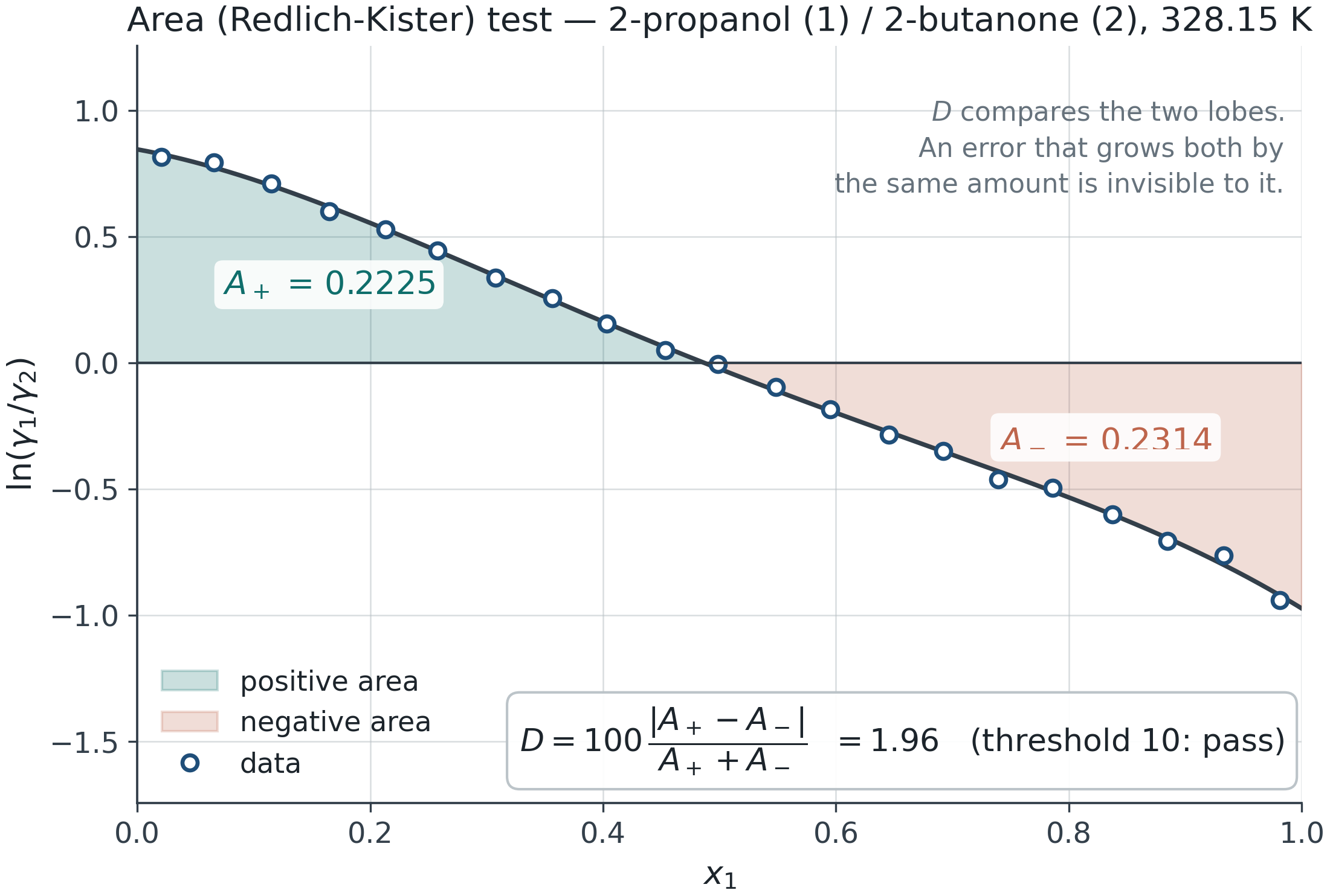
Different tests answer different questions
| Diagnostic | Evidence and limitation |
|---|---|
| Area | Global signed integral; endpoint coverage matters |
| Point/local | Local deviations; differentiation amplifies noise |
| Model-based | Deviations relative to the chosen model |
| Herington | Empirical temperature-range correction |
Agreement across tests strengthens a diagnosis but does not prove the data are correct.
Isobaric data need temperature information
At approximately constant P, \sum_i x_i\,d\ln\gamma_i=-\frac{h^E}{RT^2}\,dT
Independent excess-enthalpy data can support the temperature correction. An empirical range correction does not replace measured hᴱ.
Missing endpoints require an explicit extrapolation assumption.
Fitting objective and parameter convention
Lab 08 minimizes the mean of \left(100\frac{P_{pred}-P_{obs}}{P_{obs}}\right)^2+[100(y_{pred}-y_{obs})]^2
Compare one-parameter Margules, two-parameter Margules and NRTL on the same rows. NRTL α is fixed. This objective has no measurement-uncertainty weighting.
Residual structure matters
A lower scalar error may accompany biased residuals near an endpoint or a narrow temperature interval.
Compare residuals against composition and temperature. Report parameter bounds and temperature convention.
If a test set is available, keep it independent of fitting. Lab 08 does not provide automated cross-validation or confidence intervals.
Class demonstration · Labs 03 and 08
Consistency diagnostics · Student VLE input
- Compare a clean dataset with a controlled defect in Lab 03.
- Load Lab 08’s synthetic example and inspect its Antoine convention.
- Fit two models to identical observations and compare residuals.
Synthetic examples are training data, not experimental validation.
Guided exploration · 35 minutes
Use your dataset or the provided synthetic example.
Record source, component order, units and valid range. Compare two models. Explain one residual pattern and one unsupported extrapolation.
Save the study JSON, residual CSV and worksheet. If real data are unavailable, clearly label the synthetic case.
A fitted model has a domain
A single-temperature fit supplies composition dependence at that temperature. It does not establish dγ/dT.
A VLE fit need not identify LLE accurately. Similar VLE residuals can conceal different liquid Gibbs-energy curvature.
Session 3 adds stability and liquid coexistence evidence.
Exit question
A dataset passes an area criterion and NRTL gives a small pressure error.
Give two reasons why this is insufficient to claim accurate LLE predictions.
What additional observation or check would reduce each uncertainty?
Independent practice · suggested 60–90 minutes
One dataset, at least two activity models, residuals and a justified validity statement.
Retain the calculator export, your worksheet, a comparison plot/table and one independent check. State an assumption that limits your conclusion.
Use the core labs on the learning path. Optional extensions are additional work.
References and further study
Module reference deck · Lab sources and equations
Derivations and original figure references remain in the corresponding module deck. Each lab records its implemented equations and assumptions.
Synthetic worked examples illustrate calculations; they are not evidence of real-system accuracy.