Phase Stability and Complex Equilibria

Module 5 · 2105603 Advanced Chemical Engineering Thermodynamics

Soorathep Kheawhom

9 August 2026

 

Convergence is not correctness.

A flash calculation solves the equations it was given.
It does not check that they were the right equations.

What this module establishes

Introduction

Module 4 ended with a flash that had no way of noticing it was solving the wrong problem. This module supplies the missing test, and then follows the consequences.

The callback

Module 1 introduced mechanical stability for a pure fluid through the spinodal — the locus where (\partial P/\partial V)_T = 0 and the fluid can no longer resist a density fluctuation.

This module is the same idea in composition space, where it becomes the tangent plane criterion.

Four questions

• Where do two liquid phases come from?
• How do I test whether a computed phase is stable?
• What does a ternary split look like, and which models can produce one?
• What does all this cost a separation designer?

Stability from the Gibbs energy of mixing

PART I

Section 5.1   One curve, one tangent line, and one change of curvature.
Everything about a binary split is in that picture.

Why a liquid splits at all

5.1 · Stability from the Gibbs energy of mixing

Mixing is entropically favourable. A split needs the energetic term to defeat that, and it can only do so over part of the range.

\frac{\Delta g_{\rm mix}}{RT} = \underbrace{x_1\ln x_1 + x_2\ln x_2}_{\text{ideal, always convex}} \; + \; \underbrace{\frac{G^E}{RT}}_{\text{can be concave}}

The competition

The ideal part is convex everywhere and has infinite slope at both ends, which is why a little of anything always dissolves. A split therefore never reaches the pure vertices.

The threshold

For the symmetric case G^E/RT = A x_1 x_2, the curve first loses convexity at A = 2, at x_1 = \tfrac12. Below that value no parameter combination can produce two phases; above it, the gap opens from the middle outwards.

The picture

5.1 · Stability from the Gibbs energy of mixing

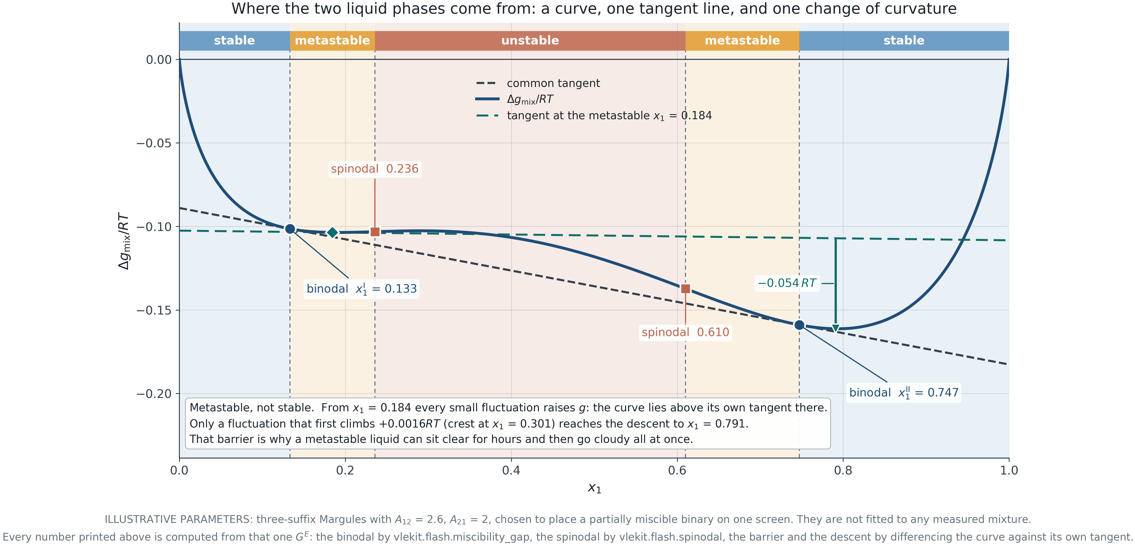
F5.1 · Binodal from the common tangent, spinodal from the change of curvature, and the metastable band between them.

Metastable is not stable, and it is not a technicality

5.1 · Stability from the Gibbs energy of mixing

Between the binodal and the spinodal a liquid is stable against small fluctuations and unstable against large ones.

Unstable

Inside the spinodal, \mathrm{d}^2\Delta g/\mathrm{d}x_1^2 < 0. Any fluctuation, however small, lowers the Gibbs energy. Separation begins everywhere at once and needs no nucleus.

Metastable

Between binodal and spinodal the curve lies above its own local tangent nearby, so a small fluctuation is resisted. In the case on the previous slide the barrier is +0.0016\,RT and the eventual descent is -0.054\,RT: a thirty-fold reward, behind a small wall.

Why it matters

A metastable liquid can sit clear for hours and then go cloudy all at once when a nucleus appears. Emulsions, supersaturated solutions and polymer blends all live in this band, and a design that assumes equilibrium will be surprised.

Tangent plane distance

PART II

Section 5.2   The common tangent works for a binary because a tangent is a line.
For three components it is a plane, and for more it cannot be drawn at all.

The criterion

5.2 · Tangent plane distance

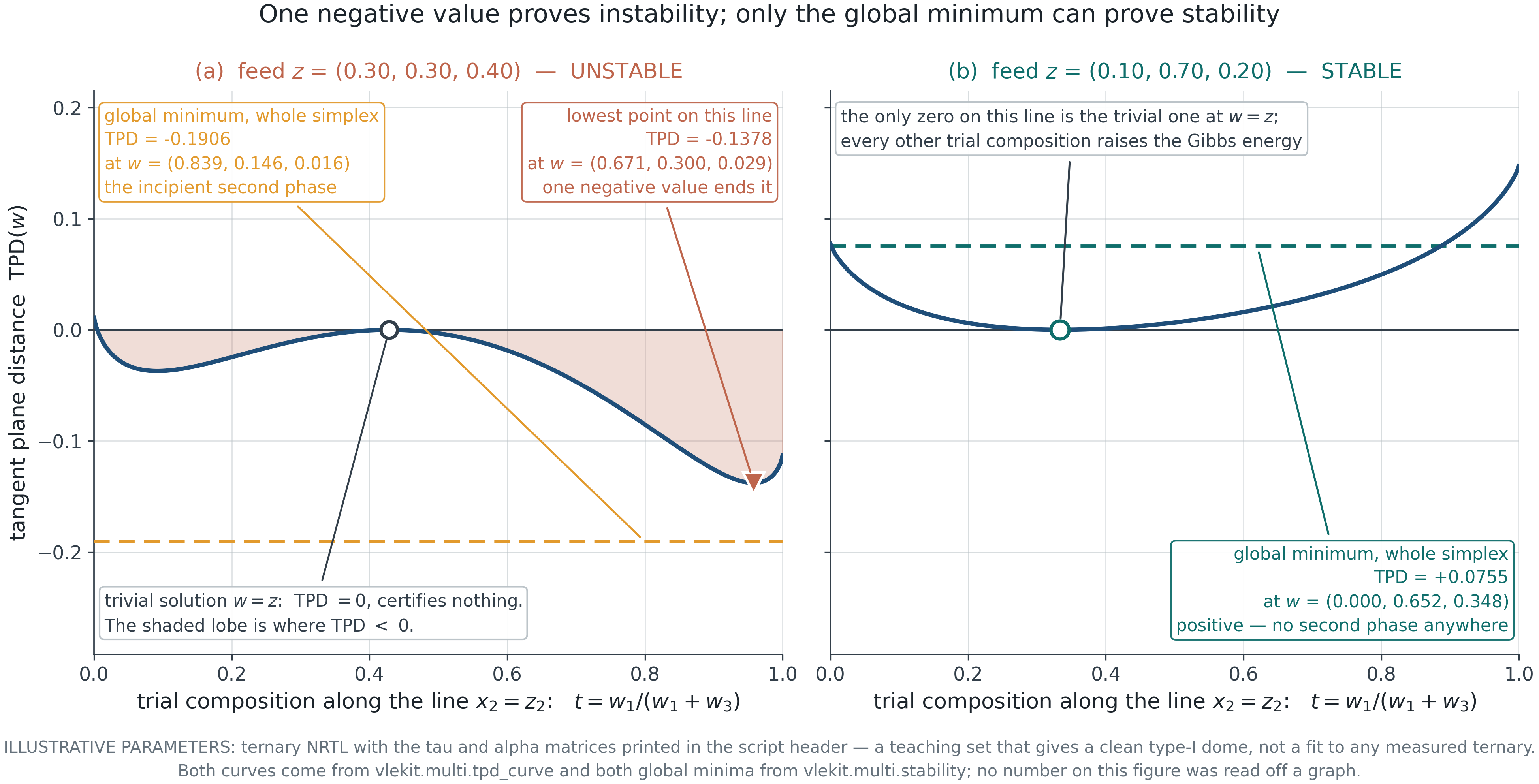
Michelsen: a phase is stable if and only if the tangent plane distance is non-negative for every trial composition.

\mathrm{TPD}(\mathbf{w}) = \sum_i w_i\left[\ln w_i + \ln\gamma_i(\mathbf{w}) - \ln z_i - \ln\gamma_i(\mathbf{z})\right]

What it measures

The vertical distance from the Gibbs energy surface at the trial composition \mathbf{w} down to the plane tangent to that surface at the feed \mathbf{z}. Negative means some other phase lies below the plane, so the feed is not the global minimum.

The asymmetry

One negative value anywhere proves instability. Proving stability requires the global minimum over the whole composition space — a much harder claim, and the reason stability analysis is a research topic rather than a formula.

What it looks like

5.2 · Tangent plane distance

F5.2 · The same criterion on an unstable and a stable feed. Note that the drawn line is a slice: the global minimum of the unstable case lies off it.

The trivial solution

5.2 · Tangent plane distance

\mathbf{w} = \mathbf{z} gives \mathrm{TPD} = 0 exactly, for every feed, stable or not. It is a stationary point and it certifies nothing.

The trap

Start the minimisation at the feed and it will sit there, return zero, and report stability. The answer looks like a converged calculation because it is one.

The remedy

Start near each pure component, and from the feed pushed halfway toward each vertex. Discard any converged trial phase that has come back to the feed. This is Michelsen’s recommendation and it is what the course code does.

Where it is used

Stability analysis runs before the flash, not after. The trial phase it returns is also the best available initial estimate for the flash that follows, so the test pays for itself.

Liquid-liquid equilibrium

PART III

Section 5.3   What a split looks like when there are three components,
and which models can produce one at all.

The ternary picture

5.3 · Liquid-liquid and vapour-liquid-liquid equilibrium

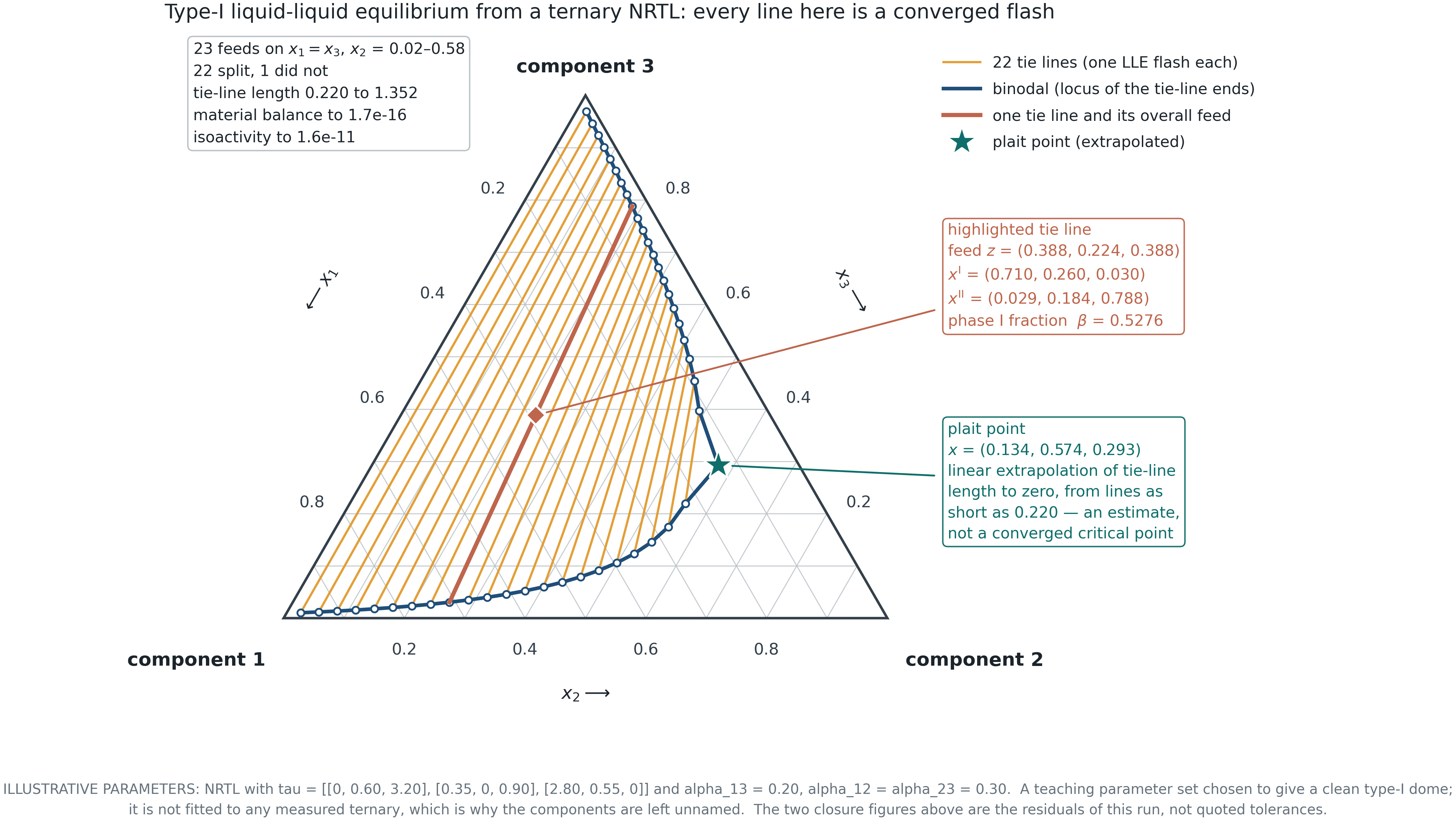
F5.3 · Type-I dome from a ternary NRTL. Every tie line is a converged flash; the plait point is an extrapolation and is labelled as one.

Why NRTL can and Wilson cannot

5.3 · Liquid-liquid and vapour-liquid-liquid equilibrium

This is a property of the functional form, argued from the G^E introduced in Module 3 — not a matter of finding better parameters.

Wilson

\frac{G^E}{RT} = -\sum_i x_i \ln\!\Big(\sum_j \Lambda_{ij} x_j\Big)

The form cannot make \Delta g_{\rm mix} lose convexity for any positive \Lambda. A sweep over thirty-six binary parameter pairs and twelve random ternary matrices produces no split — ever.

NRTL

The local-composition weighting G_{ij} = \exp(-\alpha\tau_{ij}) gives the model a second scale, and with it the ability to make G^E large and asymmetric enough to defeat the entropy of mixing. This is why every published LLE correlation uses NRTL or UNIQUAC and none uses Wilson.

Module 4 met the same limitation from the other side: fitted to a system that does split, Wilson bought the fit with an infinite-dilution activity coefficient of about twenty thousand. The absurd number was the symptom; this is the cause.

Three phases, and the counting that goes with them

5.3 · Liquid-liquid and vapour-liquid-liquid equilibrium

Vapour over two liquids is common in practice — steam distillation, azeotropic drying, any decanter on a column overhead.

F = C - \pi + 2

System	C	\pi	F	What is left free
Binary VLE	2	2	2	T and P, or T and x_1
Binary VLLE	2	3	1	Fix P and everything else is determined
Ternary LLE	3	2	3	T, P and one composition
Ternary VLLE	3	3	2	T and P; all compositions follow

Binary VLLE at fixed pressure has no remaining freedom: the temperature and all three compositions are fixed by the system. That is why a heterogeneous azeotrope boils at a single reproducible temperature.

Parameters fitted to VLE, used for LLE

5.3 · Liquid-liquid and vapour-liquid-liquid equilibrium

The extrapolation warning from Module 4, in its most expensive form.

Why it fails

VLE data constrain G^E mainly through its first derivative, over the composition range measured. A phase split is governed by the second derivative, often in a range where no VLE data exist. A parameter set can reproduce every measured bubble pressure and be wrong about whether the liquid splits at all.

What to do

If the answer depends on the split, fit LLE data — mutual solubilities are cheap to measure and pin the second derivative directly. Where both matter, fit both together and report the compromise. Never present a VLE-fitted split as a prediction without saying which data it rests on.

Azeotropy, boundaries and critical behaviour

PART IV

Section 5.4   What all of this costs a separation designer.

Two kinds of azeotrope

5.4 · Azeotropy, distillation boundaries and critical behaviour

Homogeneous and heterogeneous. The difference is worth money.

Homogeneous

One liquid phase at the azeotropic composition. y_i = x_i, no further separation by ordinary distillation, and no way around it without changing the pressure or adding an entrainer.

Heterogeneous

The azeotropic liquid is inside a miscibility gap, so the condensate splits in a decanter into two liquids of different composition — neither of which is the azeotrope. The split does the separation that distillation could not, and each layer is returned to a different column.

That is the industrial route for ethanol dehydration and for drying solvents with an entrainer.

Residue curves and the boundary

5.4 · Azeotropy, distillation boundaries and critical behaviour

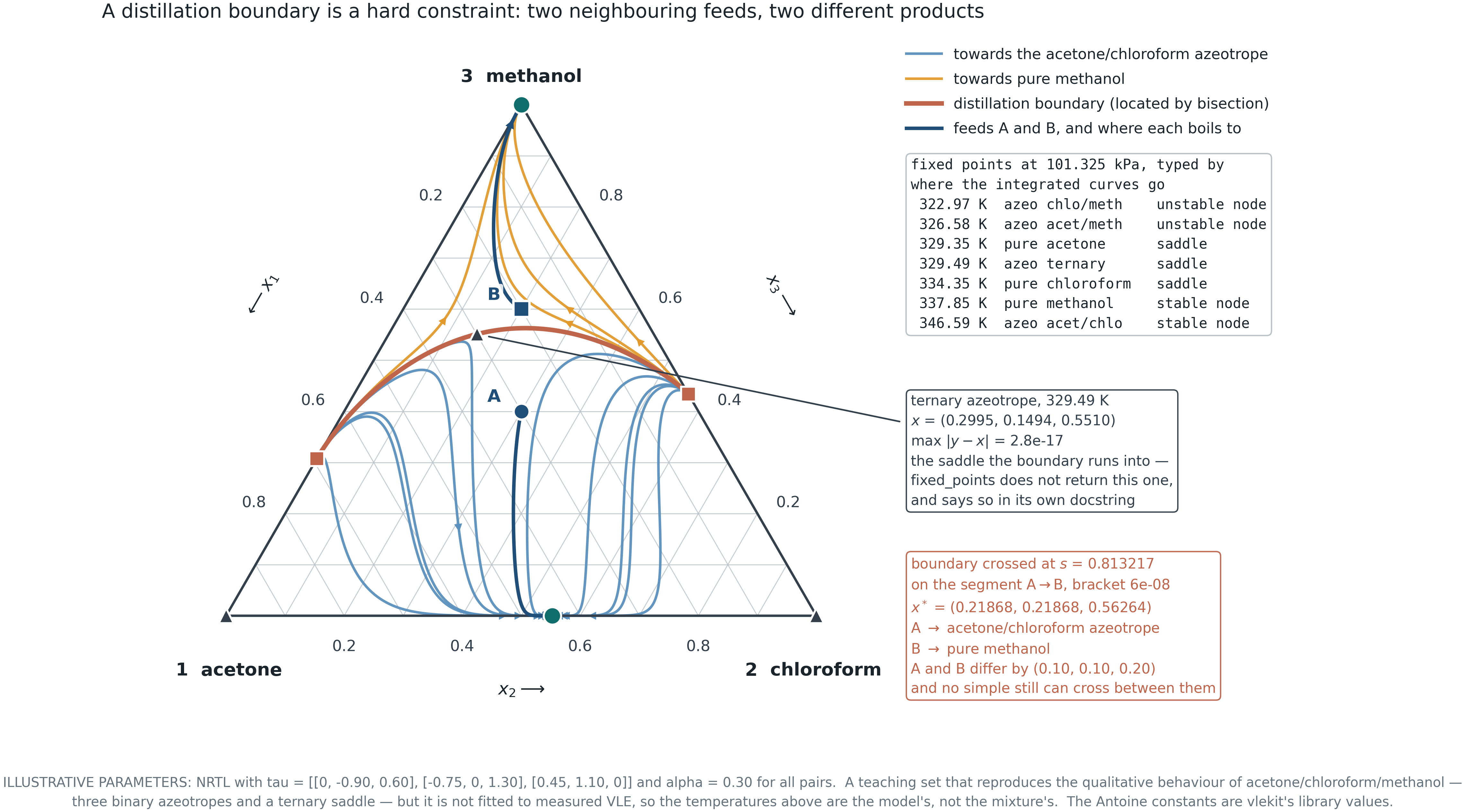
F5.4 · Residue curve map. The boundary was located by bisecting between two feeds until the end node flipped, not drawn by hand.

A saddle the search does not look for

5.4 · Azeotropy, distillation boundaries and critical behaviour

The boundary on the previous slide runs into a ternary azeotrope — a fixed point that involves all three components at once.

Why it is hard to find

The course code searches every binary edge for azeotropes by sign change, which is reliable because each edge is one-dimensional. A ternary azeotrope sits in the interior, where a sign-change scan does not generalise; finding it reliably needs a homotopy method. The code says so in its own docstring rather than returning a list that quietly misses one.

Why it matters

Interior fixed points are usually saddles, and saddles are where boundaries terminate. Miss one and the topology of the map is wrong — which means the predicted set of reachable products is wrong.

For this system it sits at x = (0.30, 0.15, 0.55) and 329.5 K, where \max|y_i - x_i| = 3\times10^{-17}.

Double azeotropy, and what actually decides it

5.4 · Azeotropy, distillation boundaries and critical behaviour

The received version is wrong

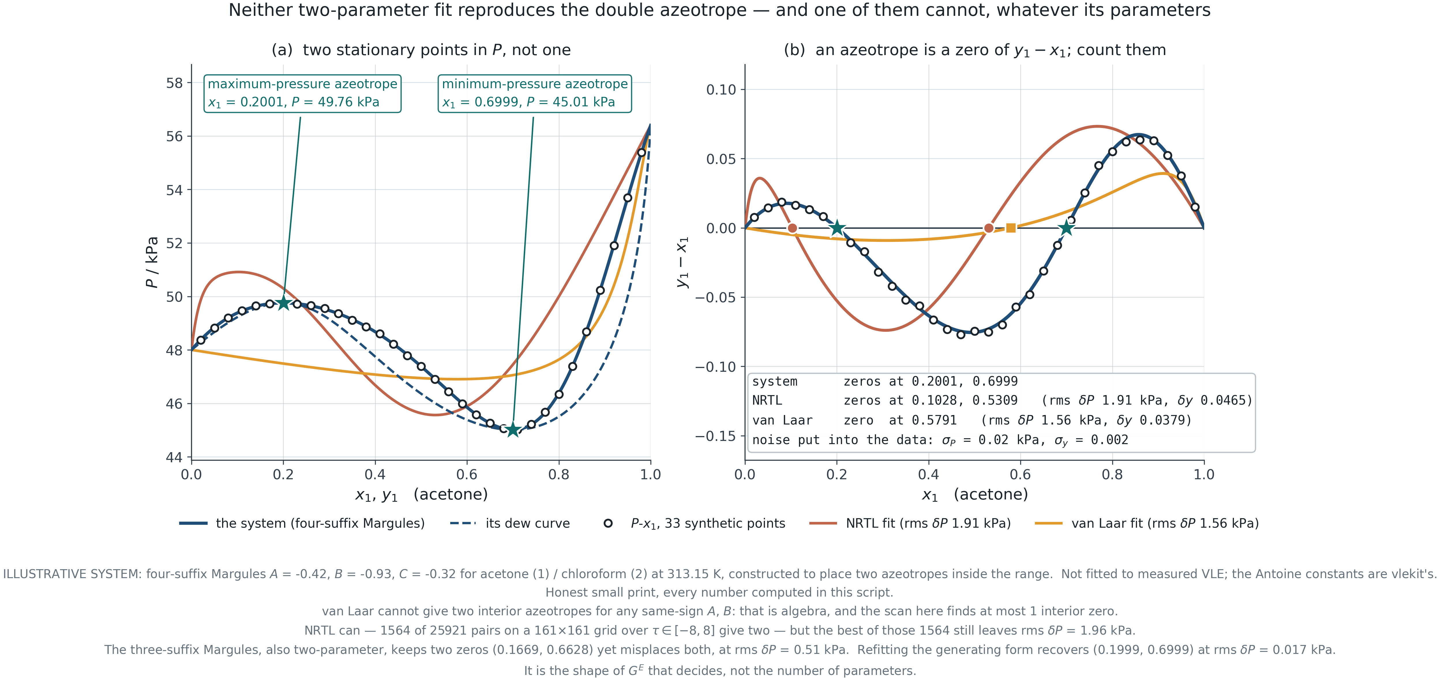
It is usually said that a two-parameter model cannot produce a double azeotrope. Van Laar indeed cannot — for same-sign parameters its \ln(\gamma_1/\gamma_2) has exactly one interior zero. But NRTL can, and so can the two-parameter three-suffix Margules.

What decides it

The shape of G^E, not the number of parameters. Here neither fitted two-parameter model reproduces the second azeotrope: NRTL misplaces both zeros and leaves an rms error a hundred times the noise.

F5.6 · An illustrative double azeotrope, with two fitted two-parameter models failing to reproduce it.

The mixture critical point is not the top

5.4 · Azeotropy, distillation boundaries and critical behaviour

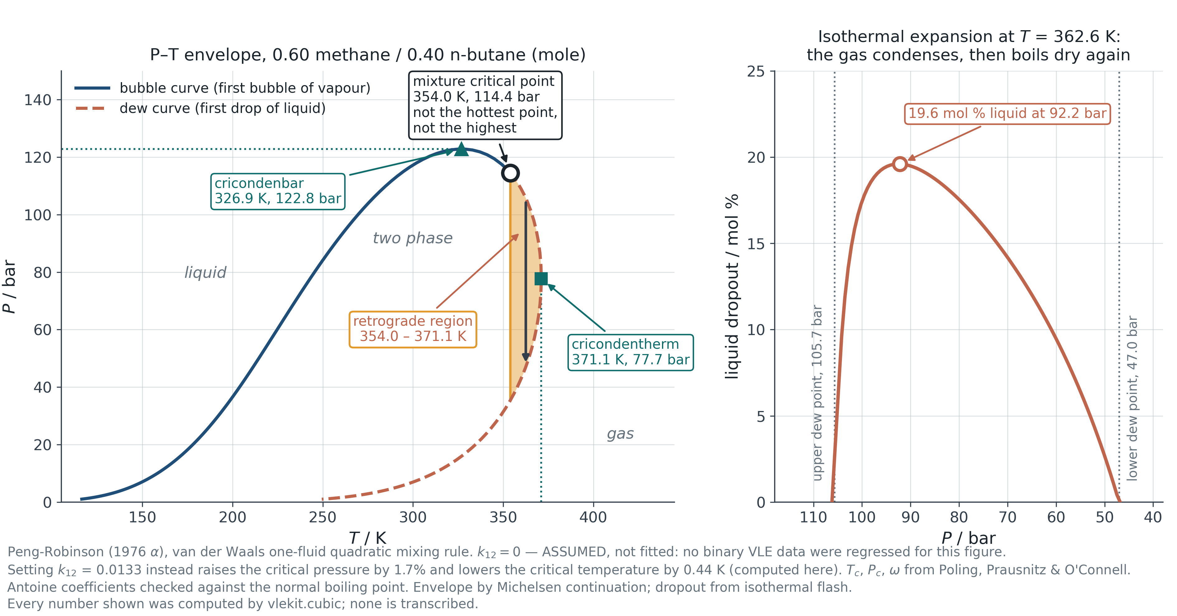
F5.5 · Peng-Robinson envelope for a light/heavy pair. Critical point, cricondentherm and cricondenbar are all different points. k_{ij} = 0, assumed and labelled.

Retrograde condensation

5.4 · Azeotropy, distillation boundaries and critical behaviour

Drop the pressure at constant temperature and liquid appears. Then keep dropping and it evaporates again.

Why it happens

Between the critical temperature and the cricondentherm the dew curve is crossed twice at one temperature. Expanding from high pressure the mixture enters the two-phase region through the upper dew point, drops out liquid, and leaves again through the lower one.

Why it costs money

Gas-condensate reservoirs sit in exactly this region. As the reservoir is produced its pressure falls and valuable heavy hydrocarbons condense in the pore space, where they are largely unrecoverable. Field development plans are built around keeping the pressure above the dew point.

What you must be able to do

Closing

The module in six statements.

1. Read a \Delta g_{\rm mix} curve. Locate the binodal by common tangent and the spinodal by curvature, and say which region a given composition is in.
2. Apply the tangent plane criterion. Compute it, interpret its sign, and explain why instability has a certificate and stability does not.
3. Distinguish metastable from unstable. And say what each means for what you would observe in a vessel.
4. Say which models can produce a split, and why. Argued from the functional form, not from a table of which ones people use.
5. Read a residue curve map. Identify the nodes, the boundary, and the products reachable from a given feed.
6. Explain retrograde condensation. Including why the critical point is not the top of the envelope.