Written companion to the video opening
First, let us answer your questions
Before solid equilibria and adsorption, clarify what a test result means and how a Gibbs graph supports a phase decision. We will define the symbols, follow one calculation and explain the result.
Choose one opening route: watch the integrated video opening, or use this written explanation with a calculator and your notebook. Both routes use the same R1–R3 questions. If you watch the opening, this page is a reference, not another required 20-minute activity. No new PDF or JSON export is required.
Written-route guide: allow about 20 minutes, including 4 minutes for R1–R3 before revealing the checks. In the video, pause at Opening 13 and check at Opening 14. The opening replaces the former required H1–H4 activity; H1–H4 is optional. Submit only the existing Session 4 form at the end of the full lesson.
Three questions need different evidence
| Question | Evidence to examine |
|---|---|
| Do the activity data satisfy a thermodynamic relationship? | Gibbs–Duhem diagnostics, with the path, assumptions, numerical method and data coverage stated. |
| Can a chosen model reproduce the observed VLE? | Predicted versus observed pressure P and vapor mole fraction y, using a defined fit and model. |
| Is this phase state stable? | The lowest possible total Gibbs energy at fixed T, P and conserved composition, within the admitted phase model. |
A fitted curve, a consistency score and a stability test answer different questions. A low number is useful only after we identify the question and its assumptions.
If D and r pass, is Gibbs–Duhem satisfied?
A pass says that the selected diagnostic met its criterion. It does not prove that every point is correct. First distinguish an integrated area, a local residual and an average score.
1. D compares positive and negative areas
Plot f(x) = ln(γ1/γ2) against liquid mole fraction x = x1. Let A+ be the area above zero and A− the positive magnitude of the area below zero.
For the isothermal case used here, with the pressure contribution neglected, the full-range signed integral should vanish. Lab 03 reports the empirical D < 5% criterion. A small D means a small net area imbalance; positive and negative errors may cancel.
2. r is a local residual; the displayed score is an average
Write gE for the dimensionless excess Gibbs energy per mole. The subscript distinguishes it from the total mixing-energy curve used later. Lab 03 calls this quantity g in its differential formula:
For this isothermal approximation, an exact consistent relation gives r = 0. A nonzero numerical residual can reflect inconsistent input, differentiation error or noise. The Lab averages the absolute residuals at interior points and applies the teaching threshold score < 5.
The score is dimensionless, not a percentage error. Multiplying by 100 does not create a relative-error denominator. A small average can hide a narrow local peak, so inspect the residual curve too.
Concrete example: at 350 K, choose the localized defect, amplitude 0.25 and 81 points. The Lab gives D ≈ 1.956% and score ≈ 1.591, both below their limits, but r(0.35) ≈ −0.250. The localized departure remains visible even though both summaries pass.
Optional: reproduce this example in Lab 03
This is a brief comparison, not another assignment. No export is needed.
- Open Lab 03: consistency tests.
- Set Data set → Synthetic · isothermal, 350 K, Controlled perturbation → Localized defect near x₁ = 0.35, Amplitude → 0.25 and Sampling resolution → 81 points.
- Read the area and differential scorecards. Under Inspect, choose Local Gibbs–Duhem residual. Find the peak near x = 0.35.
- Explain aloud: “The average meets its threshold, but a local departure remains.” Return to this page.
Optional: why did 41 versus 161 points change D only slightly?
| Points | D (%) | 100 mean |r| |
|---|---|---|
| 41 | 2.013463 | 1.671839 |
| 81 | 1.956058 | 1.590767 |
| 161 | 1.941724 | 1.565607 |
These are denser samples of the same synthetic function, not new experiments. The narrow defect remains. More points can improve numerical integration and reveal the residual shape, but do not remove the defect or force the average to fail. This comparison does not establish a universally sufficient number of experimental points.
The plotted residual uses three-point numerical derivatives. It is a teaching diagnostic, not the NIST Padé-based Kojima point-test implementation. Isobaric data also need the appropriate temperature/excess-enthalpy correction; do not apply the simplified isothermal formula indiscriminately.
Optional: where does the residual equation come from?
Differentiate the excess Gibbs expression using the product rule:
At fixed temperature and pressure, Gibbs–Duhem requires the last two terms to sum to zero. Subtracting ln(γ1/γ2) leaves the residual r. This explains why r should vanish for exact consistent activity functions under those conditions.
For an isobaric path with changing temperature, the Lab adds the term [HE/(RT²)] dT/dx, where HE denotes the molar excess enthalpy; a verdict needs that information. The pressure/excess-volume term is neglected in this teaching implementation.
The Herington alternative uses the empirical allowance J = 150(Tmax − Tmin)/Tmin, with both temperatures in kelvin; J is dimensionless. It compares D − J with 10. J is not a measured excess enthalpy. Do not interchange isothermal and isobaric criteria.
The full-area test also needs the full composition interval. Extrapolated endpoints make the result conditional. If A+ + A− vanishes, D is undefined, not automatically failed.
3. Where does the Van Ness test fit?
It is a modeling-capability approach within thermodynamic consistency testing. Lab 03 uses a Van Ness-type teaching variant: a consistent NRTL activity model is fitted jointly to P and y at the observed temperature and liquid composition.
The limits are Δp < 1% and Δy < 1 percentage point (an absolute mole-fraction difference below 0.01 on average). The second is not a relative percentage error in y.
Meeting both limits establishes reproduction by this model under these assumptions. It does not certify every measurement. Missing a limit can reflect model flexibility, property correlations or experimental data. This fit is not the full NIST TDE implementation.
Method references: NIST area and Herington tests · NIST point test · NIST Van Ness modeling test. The Lab states where its teaching methods differ.
How can I decide stability without a badge?
First read what the graph represents. At fixed T and P, let x be a possible liquid composition and z the overall composition of our material. The curve gives the Gibbs energy if that composition is kept as one homogeneous liquid.
The first two terms are ideal mixing. The last is the symmetric Margules excess contribution. This g is total dimensionless mixing Gibbs energy, not the excess-only gE in the consistency formula above.
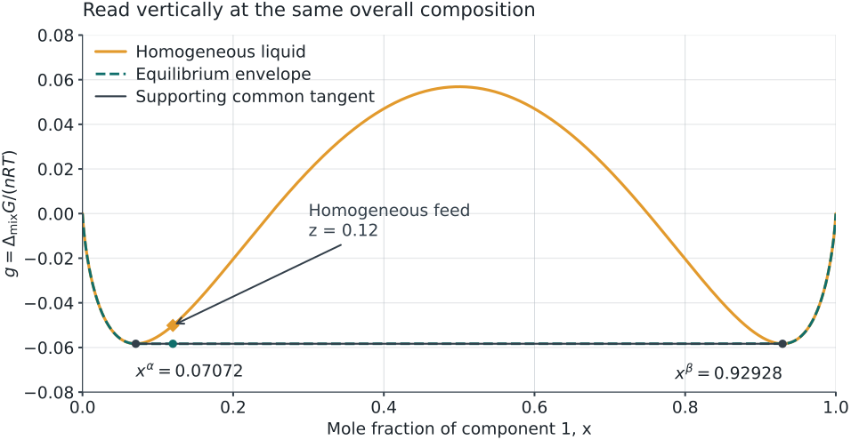
- Amber curve, “Homogeneous liquid”: evaluate the equation at each trial composition x. Its height is the single-liquid mixing Gibbs energy.
- Two contact compositions: xα = 0.07072018 and xβ = 0.92927982. They are candidate coexisting phase compositions, not phase amounts.
- Graphite common tangent: a line ℓ(x) touching at both contacts. Here it is horizontal because this example is symmetric; common tangents need not be horizontal in general.
- Dashed teal equilibrium envelope: the lowest admissible Gibbs energy. Between the contacts it follows the supported two-liquid line; outside this interval it follows the stable single-liquid branch for this model.
- Two feed markers at z = 0.12: the amber diamond marks the homogeneous liquid on the curve; the teal circle marks the two-liquid state on the common tangent below it. Compare their heights at the same composition. Their vertical difference is the Gibbs-energy reduction upon splitting. The diagonal annotation arrow only identifies the split-state point.
Step 1. Check local curvature
Positive curvature means the homogeneous liquid resists infinitesimal composition fluctuations. It does not exclude a lower-energy split into substantially different compositions.
Step 2. Compare an admissible two-liquid state
Use the two contacts and conserve total composition. Fractions here are moles of each phase divided by total moles:
The split is lower by 0.00821636 RT per mole of feed. This homogeneous feed is metastable: locally resistant to small fluctuations, but not the global minimum. The sign of either Gibbs value alone cannot decide stability; compare admissible alternatives at the same constraints and reference state.
Step 3. Check the whole composition range
Equal chemical potentials identify a candidate coexistence condition. To establish global stability in this liquid model, its common tangent must support the full curve:
A line that crosses above the curve somewhere fails this check. Comparing one pair alone can establish that the feed is not globally stable, but does not by itself establish that this pair is the global minimum. Inspect the full support condition, with numerical resolution and tolerance stated, rather than trusting a label alone.
Decision sequence: negative local curvature identifies an unstable homogeneous feed. Positive local curvature plus a lower supported split identifies a metastable feed. A homogeneous state is globally stable only when no admissible alternative lowers Gibbs energy. Zero curvature needs further examination.
Change the overall composition, then check what moves
At the same T, P and model, change only z from 0.12 to 0.35, still between the contacts:
| Overall z | xα | xβ | fβ | Homogeneous-feed curvature |
|---|---|---|---|---|
| 0.12 | 0.07072018 | 0.92927982 | 0.057398 | +3.469697: locally stable |
| 0.35 | 0.07072018 | 0.92927982 | 0.325289 | −1.604396: locally unstable |
The phase compositions stay fixed; the relative amounts change. The contact points are selected by equilibrium at the fixed conditions. The material balance selects where the overall composition lies between them.
Optional: compare the calculation in Lab 04
- Open Lab 04: liquid stability. Set Liquid model → Margules · 1 parameter and Interaction parameter A → 3.
- Set Feed mole fraction z₁ → 0.12 and press Find equilibrium. Compare the local curvature, the two phase compositions, the phase fractions and the Gibbs reduction with the calculation above.
- Under View, select Gibbs energy & common tangent to compare the curve and line. Then select Tangent-plane distance · feed stability. A negative feed TPD somewhere rejects global stability of the homogeneous feed. This is different from the Common-tangent residual (binodal construction), which checks the coexistence equations, not global support. Explain which tangent each test uses.
- Change only z₁ to 0.35 and press Find equilibrium again. Check that the contact compositions stay fixed while the phase fractions change. No additional export or submission is needed.
The graph shows equilibrium possibilities, not a nucleation barrier, separation rate or elapsed time. For further optional practice, use the existing Gibbs review video with Lab 04 demonstration.
Three short answers before Week 4
Write R1–R3 in your notebook. Use one or two sentences for each, plus the requested fraction. Keep your first answer, then add a correction if needed. These are practice checks, not another submission.
- R1. D and the mean residual score both meet their limits, but the residual curve has a narrow peak. Can you conclude that every point satisfies Gibbs–Duhem? What should you inspect?
Reveal R1 check after writing
No. Integrated or averaged summaries can hide cancellation or localized departures. Inspect the residual shape, assumptions, data coverage and numerical sensitivity. State which criterion passed instead of certifying every point.
- R2. At A = 3 and z = 0.12, g″ is positive but a supported split has lower Gibbs energy. Is the homogeneous feed globally stable, metastable or locally unstable? Give the reason without using the Lab badge.
Reveal R2 check after writing
Metastable. Positive curvature gives local resistance to small composition fluctuations, but the admissible supported split lowers Gibbs energy by 0.00821636 RT per mole of feed. The homogeneous state is not the global minimum.
- R3. Move z to 0.35 on the same supported tie line. What stays fixed? Calculate fβ. Then state why Week 4 will still need material balances after writing an equilibrium relation.
Reveal R3 check after writing
The phase compositions remain xα = 0.07072018 and xβ = 0.92927982. The lever rule gives fβ = 0.325289 and fα = 0.674711. Equilibrium specifies coexistence conditions; total inventories determine phase amounts. In Week 4, we must also check whether enough material remains for a solid phase to be present.
Now continue Week 4: open the existing worksheet at page 1, A1–A3 and continue to core slide 1. If you used this written route, skip the recorded opening using the link below. H1–H4 remains optional this week. Complete the existing Session 4 exit ticket and feedback once at the end of the required lesson.
Continue to the core lesson · skip the opening already completed
Return to the Week 4 study route · Open the existing worksheet