Liquid stability, LLE and VLLE
After midterm · Session 3 of 6 · 180 minutes
30 September 2026
Session outcome
Use global Gibbs-energy support to assess candidate liquid phases.
Before class: Review gmix, local curvature and the distinction between stationary and globally stable states.
The 180-minute class
| In class | Minutes |
|---|---|
| Recall and prediction | 10 |
| Concepts and derivation | 45 |
| Worked example | 30 |
| Break | 10 |
| Instructor lab demonstration | 25 |
| Guided student exploration | 35 |
| Discussion and interpretation | 15 |
| Exit question and independent task | 10 |
Phase equilibrium includes stability
Equality of chemical potentials identifies stationary candidate states. Stable equilibrium requires the lowest admissible total Gibbs energy.
g_{mix}/RT=\sum_i x_i\ln x_i+g^E/(RT)
A split can lower G even when a homogeneous liquid is locally stable.
Binodal and spinodal
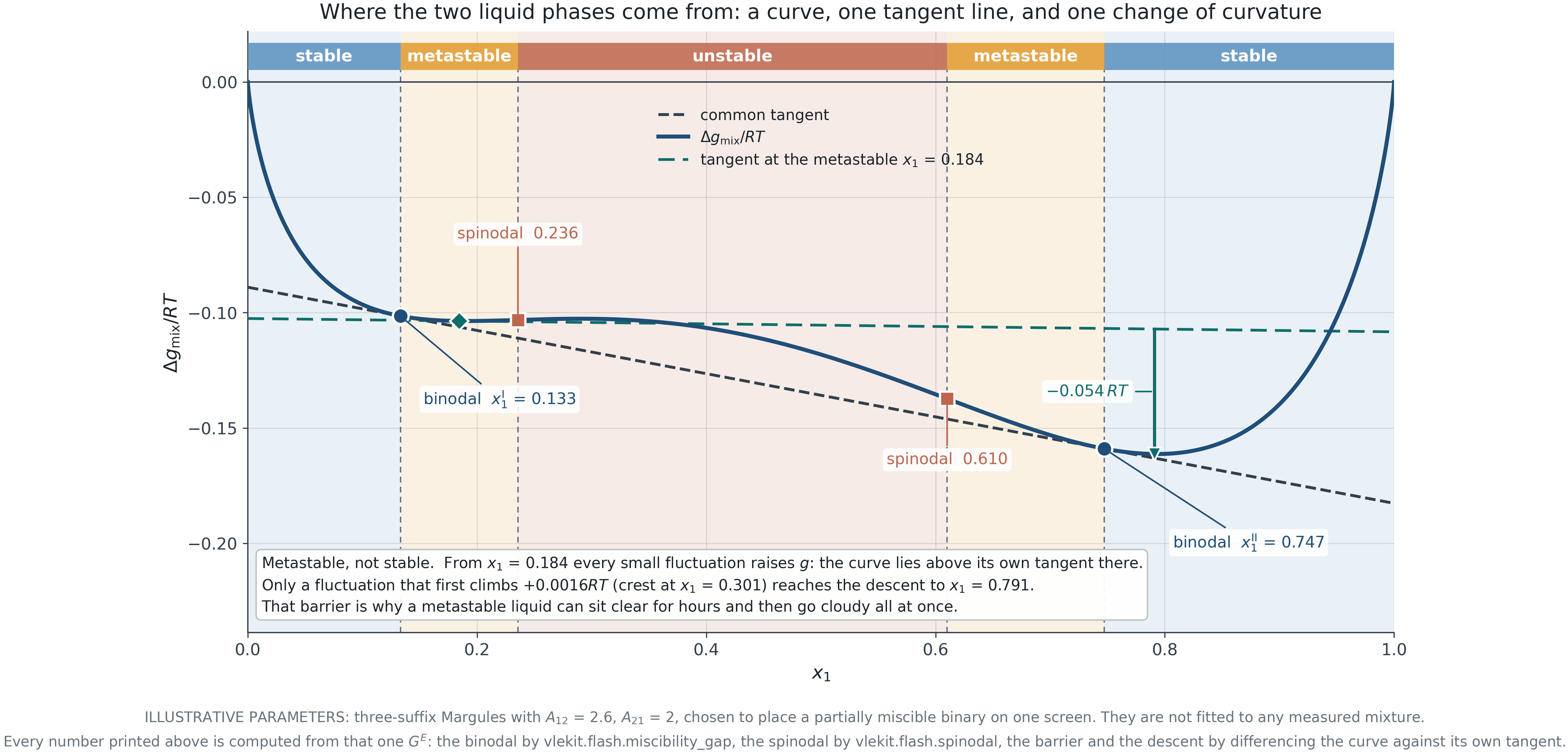
The common-tangent conditions
g'(x^\alpha)=g'(x^\beta)=\frac{g(x^\beta)-g(x^\alpha)}{x^\beta-x^\alpha}
The tangent must not lie above g(x) anywhere in the admitted composition interval.
A trivial root xᵅ=xᵝ does not establish two distinct liquid phases.
Tangent-plane distance
For a trial composition w relative to reference z, TPD(w;z)=g(w)-g(z)-g'(z)(w-z)
A negative value identifies a Gibbs-energy-lowering perturbation. Local curvature examines only the neighborhood of z.
Lab 04 evaluates the binary model; it is not a general multicomponent TPD package.
A lever-rule calculation
Synthetic tie line: x₁ᵅ=0.2, x₁ᵝ=0.8. Feed z₁=0.5.
f_\beta=\frac{z_1-x_1^\alpha}{x_1^\beta-x_1^\alpha}=0.5
For z₁=0.35, fᵝ=0.25. At the same coexistence conditions, the phase amounts change but the tie-line endpoints do not.
Model shape and liquid splitting
Positive activity deviations alone do not guarantee LLE. The mixing Gibbs-energy shape must support a split.
The labs include Margules and NRTL options with different shapes. Standard Wilson behavior is discussed in the reference deck, not implemented as an LLE solver here.
LLE fitting uses different evidence
Tie-line data constrain the coexistence compositions. Fitting must reproduce distinct phases and a supported common tangent.
A small tie-line error at one T does not establish a unique parameter set or a temperature law.
Lab 05 retains the input observations and checks stability of the fitted result.
Class demonstration · Labs 04 and 05
Stability and LLE · LLE fitting
- Compare convex and nonconvex mixing Gibbs curves.
- Inspect global support and the phase fractions.
- Fit a tie-line example at its stated temperature and inspect the stability check.
Guided exploration · 35 minutes
Choose one state with a supported liquid split.
Predict the effect of changing z while holding T and model fixed. Record phase compositions and amounts, then check the lever rule.
Use a fitting example to state one parameter uncertainty that a small residual cannot resolve.
Vapor–liquid–liquid coexistence
\hat f_i^V=\hat f_i^{L\alpha}=\hat f_i^{L\beta}
For a binary nonreacting system with three phases, the phase rule gives one intensive degree of freedom before imposing T or P.
Phase compositions and phase amounts are different unknowns. Specifying T and P does not always uniquely determine all amounts.
Three phase amounts can form a family
Given three fixed binary phase compositions, f_\alpha+f_\beta+f_V=1 z_1=f_\alpha x_1^\alpha+f_\beta x_1^\beta+f_Vy_1
There are two independent constraints on three fractions. Nonnegativity bounds the feasible family. Another independent extensive constraint may select a member.
VLLE extension
Compare the supported liquid and vapor states. Move within the admissible phase-fraction family and verify the overall balance.
Identify a state where the vapor fraction is constrained by nonnegativity. Explain why equal fugacities alone cannot determine every fraction.
Where the model can be reused
A fitted liquid model needs a matching component order, parameter convention and temperature before reuse.
VLE also requires pure-component vapor pressures and a vapor model. LLE experimental pressure is not a vapor-pressure correlation.
A new phase calculation brings new assumptions and validation needs.
Exit question
A solver reports two liquid compositions with equal chemical potentials and a tiny residual.
What checks distinguish a real stable split from a trivial or metastable result?
Which quantities change when only the overall composition changes?
Independent practice · suggested 60–90 minutes
A common-tangent result, one lever-rule check and one limitation of the fitted parameters.
Retain the calculator export, your worksheet, a comparison plot/table and one independent check. State an assumption that limits your conclusion.
Use the core labs on the learning path. Optional extensions are additional work.
References and further study
Module reference deck · Lab sources and equations
Derivations and original figure references remain in the corresponding module deck. Each lab records its implemented equations and assumptions.
Synthetic worked examples illustrate calculations; they are not evidence of real-system accuracy.