Solid equilibria and adsorption
After midterm · Session 4 of 6 · 180 minutes
30 September 2026
Session outcome
Distinguish pure-solid SLE, bulk sublimation and surface adsorption.
Before class: Review chemical potentials, fusion/sublimation data and absolute versus excess adsorption.
The 180-minute class
| In class | Minutes |
|---|---|
| Recall and prediction | 10 |
| Concepts and derivation | 45 |
| Worked example | 30 |
| Break | 10 |
| Instructor lab demonstration | 25 |
| Guided student exploration | 35 |
| Discussion and interpretation | 15 |
| Exit question and independent task | 10 |
Bulk and surface equilibria
| Problem | Equilibrium description |
|---|---|
| SLE | Solute chemical potential equal in liquid and solid |
| Bulk GSE | Chemical potential equal in gas and solid |
| Adsorption | Surface loading at gas/solution chemical potential |
Surface uptake is not the formation of a macroscopic bulk solid phase.
Pure-solid solubility
Neglecting fusion heat-capacity corrections for a pure solid, \ln(x_i\gamma_i)=-\frac{\Delta H_{fus,i}}{R}\left(\frac1T-\frac1{T_{m,i}}\right)
The standard state is the subcooled pure liquid. The solid is present with unit activity. A solid solution requires a different solid-phase model.
A solubility hand calculation
Synthetic input: Tₘ=350 K, ΔHfus=10 kJ/mol and T=300 K.
For an ideal liquid, x^{sat}=\exp\left[-\frac{10000}{R}\left(\frac1{300}-\frac1{350}\right)\right]\approx0.564
A nonideal γ changes the required liquid composition. A value of xγ alone does not specify phase amounts.
Binary eutectic assumptions
Each pure-solid branch imposes its own solubility equation. Their intersection gives the eutectic within the admitted model.
The phase amounts follow material balances. The presence of two possible solids does not mean both occur for every overall composition.
Lab 10 excludes solid solutions and chemical reactions.
Sublimation and vessel inventory
At fixed T, a present bulk solid fixes the ideal-gas partial pressure at its sublimation pressure within the model.
In a rigid vessel, n_g^{sat}=\frac{P_{sub}(T)V}{RT}
If total subliming-species inventory is below this amount, the solid is exhausted and pressure falls below Psub.
A gas–solid inventory check
Synthetic example: T=300 K, V=1 L, Psub=10 kPa.
n_g^{sat}=10/(8.31446\times300)\approx0.00401\ \mathrm{mol}
With 0.01 mol total, about 0.00599 mol remains solid. With 0.002 mol total, no solid remains and P≈4.99 kPa.
Fixed T,V equilibrium minimizes Helmholtz energy, not Gibbs energy at fixed P.
Adsorption isotherm assumptions
| Model | Form | Interpretation/domain |
|---|---|---|
| Henry | q=KᴴP | Dilute limit |
| Langmuir | q=qₛbP/(1+bP) | Idealized finite sites |
| Freundlich | q=KPᵐ | Empirical range, no plateau |
| BET | Multilayer expression | Requires P/P₀ and a fitting window |
A better fit alone does not establish the microscopic mechanism.
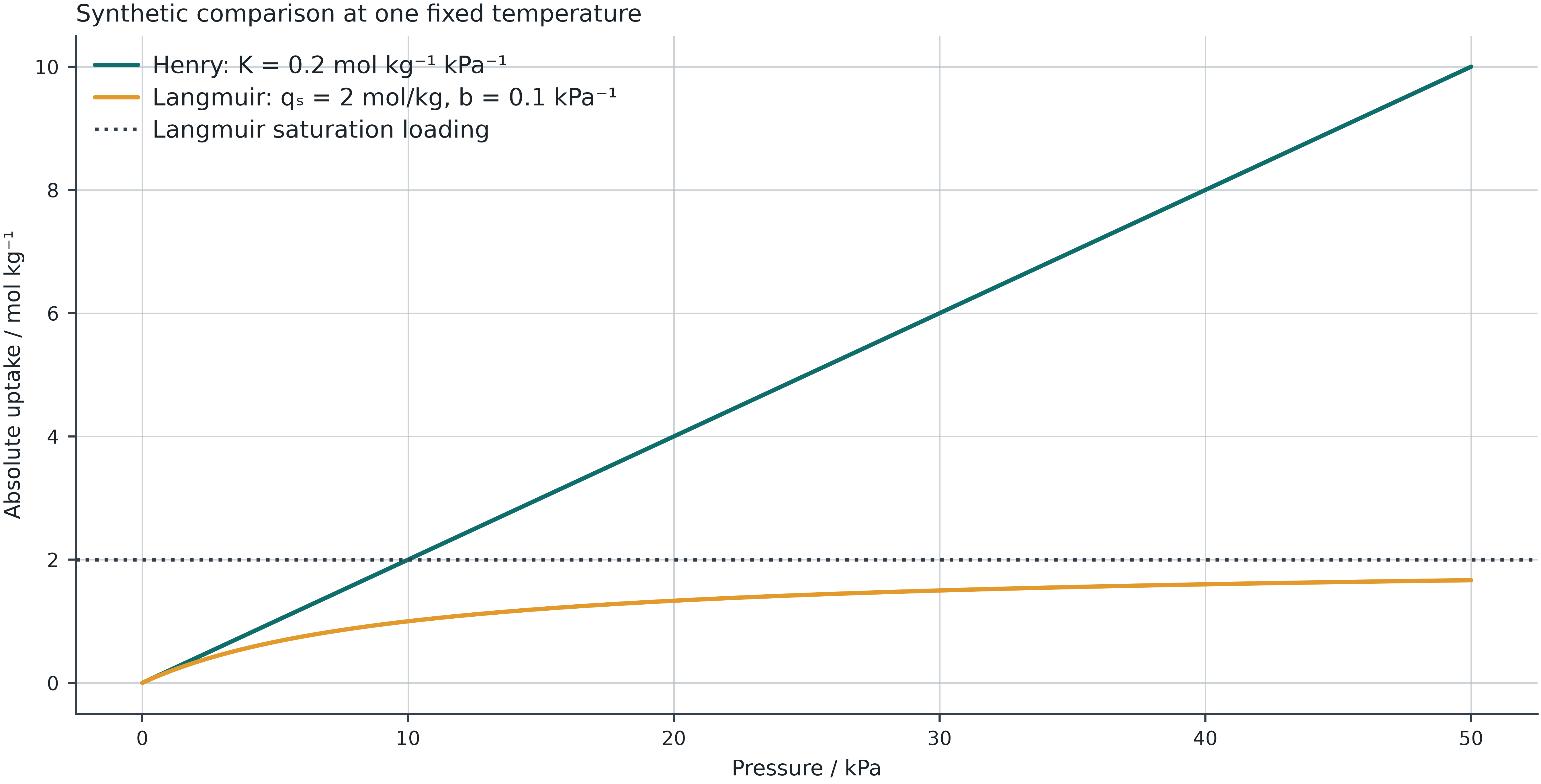
Low-pressure agreement and saturation
A closed adsorption vessel
For an ideal gas and absolute uptake q, n_{total}=\frac{PV_g}{RT}+m_s q(P,T)
Gas amount and adsorbed amount must sum to inventory. Vg is the accessible gas volume.
Excess adsorption needs a volume/density convention and cannot be substituted for absolute q without conversion.
Isosteric heat uses common loading
For the ideal-gas pressure convention, Q_{st}=-R\left(\frac{\partial\ln P}{\partial(1/T)}\right)_q
Compare pressures at the same absolute loading across temperatures. Interpolation is limited to common measured loading.
An isotherm fit does not justify extrapolated heat estimates outside overlap.
Class demonstration · Labs 10 and 11
- Cross the bulk-solid exhaustion boundary in a rigid vessel.
- Compare low-pressure Henry and Langmuir behavior.
- Inspect a closed adsorption-vessel inventory balance.
Predict what changes before each calculation.
Guided exploration · 35 minutes
Use one bulk gas–solid case and one adsorption case.
Record the fixed variables, remaining solid or surface loading, and material balance. Explain why the same phrase “gas–solid” does not imply the same model.
If fitting, retain the selected range and uptake convention.
Independent extension
Compare SLE with ideal and nonideal liquid activity. Identify how liquid nonideality changes a solubility branch.
Alternatively, examine Qst only where isotherms overlap in measured loading. Report the interpolation range and do not label extrapolation as measured evidence.
Exit question
Why can adding more bulk solid leave the gas pressure unchanged, while adding adsorbent to a closed vessel can change it?
Which phase or capacity limit ends each behavior?
Independent practice · suggested 60–90 minutes
Compare a bulk gas–solid result with adsorption; close the appropriate inventory balance and state assumptions.
Retain the calculator export, your worksheet, a comparison plot/table and one independent check. State an assumption that limits your conclusion.
Use the core labs on the learning path. Optional extensions are additional work.
References and further study
Module reference deck · Lab sources and equations
Derivations and original figure references remain in the corresponding module deck. Each lab records its implemented equations and assumptions.
Synthetic worked examples illustrate calculations; they are not evidence of real-system accuracy.