Resources
Methods, tools, and shared files for the group — from designing the question to modelling the mechanism and reporting the result.
Experimental design
How we plan experiments — start from what you want to know, then let the question set the design.
Start from the question, not the technique
The habit the group is built on: decide what you want to know, phrase it so it could come out either way, and choose the experiment that most directly separates the possible answers. Use the AI prompt pack to think a design through — or to check a write-up. Worked case studies will be added here over time.
Design the experiment from the question, not from the instrument. Decide what you want to know first; the right experiment is whatever separates the possible answers most directly. A technique you happen to have is not a reason to run it.
- State the question so it can come out either way. "Does the additive suppress dendrites?" is answerable; "characterise the additive" is not. If no result would surprise you, there is no question yet.
- Write down the prediction and its alternative. What do you expect to see, and what would the competing explanation predict instead? Two named outcomes on paper before any cell is built.
- Name the result that would change your mind. A claim that no measurement could contradict is not worth measuring. Decide, in advance, what would falsify your prediction — that observation is the experiment.
- Choose the minimal design that tells those outcomes apart. Vary one thing, hold the rest fixed, and make sure the two predictions land in visibly different places. Extra conditions that cannot change the conclusion are decoration.
- List the controls that rule out the boring explanation. Baseline, reference, and "nothing changed" conditions exist to kill the trivial reasons your effect might appear. If a reviewer can explain your result without your hypothesis, add the control that closes that door.
- Fix what you will measure and report before you start. Choose the metrics, the conditions to disclose, and the number of cells up front — not after seeing the data. This is also where the reporting checklist (below) comes in.
- Battery reporting checklist — what a battery result must disclose to be trusted and compared (below).
- Case studies (coming) — worked examples from the group: the question, the design chosen, and why.
Battery reporting checklist — what to report, what to do
Before you plot a battery result, make sure it can be trusted and compared. This is a simple summary of what every battery figure and Methods section must disclose, distilled from the reporting guidelines of Joule, ACS Energy Letters, Advanced Energy Materials, and the Nature journals — the same items most journals expect.
A reader should be able to rebuild your cell and reproduce your plot from the Methods and SI alone, and compare your numbers to anyone else's on equal terms. If they can't, something below is missing. Full version and printable copy: download the file at the bottom.
- Cell type & configuration; half-cell vs full-cell
- 2- or 3-electrode — use 3-electrode to get a single electrode's true potential / separate anode from cathode
- Counter/reference (e.g. Li) — half-cell CE ≠ full-cell CE
- Number of cells (n) — ≥3 independent cells per condition where feasible
- Active-material mass and loading (mg cm⁻²)
- Electrode area and areal capacity (mAh cm⁻²)
- Formulation (active:conductive:binder), thickness, density
- N/P ratio for full cells; Li excess for Li-metal
- Composition and amount — E/C ratio (µL mAh⁻¹). A flooded cell hides poor efficiency
- Separator type/thickness
- Voltage window (cut-offs)
- C-rate and current density; define what 1C means
- Basis of specific values: per active / electrode / cell
- Temperature (controlled?); formation, CC–CV, rests; cycle count
- Specific capacity with basis stated
- Initial & steady-state CE to enough sig-figs (99.92 %, not ~100 %)
- Retention: % over N cycles and absolute capacities
- Energy/power density — state the level; rate capability
- Test at a practical mass loading (mAh cm⁻² range) — thin electrodes inflate rate & cycling
- Run a fair control under identical conditions in the same study
- ≥3 independent cells per condition: report n, show error bars/spread, give the average — not the best cell
- Show raw voltage profiles, not only capacity-vs-cycle
- Make a full cell (or say you didn't) before claiming device-level performance
- Scalar numbers (capacity, CE, retention) as mean ± SD with n — e.g. "148 ± 4 mAh g⁻¹ (n = 3)"
- GCD voltage curves: show one representative cell (closest to the mean) — never point-by-point average voltage–capacity curves; it smears the plateaus. Overlay all cells faintly if you want to show spread
- Capacity/CE vs cycle: plot the mean with a ± SD band, or all cells thin + mean bold — not only the best
- Bar/rate summaries: bar = mean, error bar = SD, overlay individual points
- Account for every cell — how many assembled vs included; say why any were excluded
Big areal capacity from a tiny loading · half-cell shown as a full cell · CE quoted as "~100 %" · no electrolyte amount · "high rate" from an unrealistically thin electrode · only % retention with no absolute numbers · only the single best cell.
Distilled from the reporting guidelines of Joule (Battery Checklist required at submission), ACS Energy Letters, Advanced Energy Materials, and the Nature journals — which most journals, including Materials Today Energy, expect too. Full sources are in the download.
GITT & PITT — what they measure, how to run & calculate
Two intermittent titration techniques for insertion electrodes. What each one answers (diffusion coefficient, OCV, resistance vs SOC), how to design the pulses/steps, the actual equations, and the caveats — the absolute diffusion coefficient is only a relative measure. Includes references for students to read.
Both techniques step the cell a little and wait, right across the state of charge, and return the chemical (apparent) diffusion coefficient of the working ion, the equilibrium (OCV) curve, and the resistance vs SOC. The absolute D is only trustworthy for comparing samples measured the same way — see the caveats.
| GITT | PITT | |
|---|---|---|
| Diffusion coefficient D vs SOC | ✔ | ✔ |
| Equilibrium potential / OCV (thermodynamics) | ✔ | ✔ |
| Overpotential & internal resistance | ✔ | indirect |
| Solid-solution vs two-phase reaction | partly | ✔ (transient shape) |
| Resolution near a plateau | coarse | ✔ fine |
Run: constant-current pulses (~C/20–C/10, 5–30 min) each followed by a rest to equilibrium (1–10 h, until dV/dt is flat). Keep current small & pulse short so E is linear in √t. Do charge and discharge.
Read four voltages per step: ΔEs = equilibrium change (E4−E1); ΔEτ = transient change during the pulse, IR removed (E3−E2).
D = (4 / π·τ) · ( m_B · V_M / (M_B · S) )² · ( ΔE_s / ΔE_τ )² [ valid for τ ≪ L²/D ]
τ pulse time · m_B, M_B mass & molar mass of active material · V_M molar volume · S electrode–electrolyte area. Also: OCV = rested voltage; overpotential η = Emeas − Eeq; internal resistance R = η / I.
Run: a staircase of small steps (ΔE ≪ 25 mV, typically 5–20 mV); hold each until the current decays to a cut-off, then step again. Integrate current per step → dQ/dE and OCV.
Long time (t ≳ L²/D):   ln I(t) = const − (π²D / 4L²)·t   →   D = −(4L²/π²)·slope
Short time (t ≪ L²/D):  I(t) ∝ t^(−1/2)   (Cottrell)     →   D from slope with ΔQ and L
L = diffusion length (particle radius / film thickness). Bonus: current decays monotonically for solid-solution insertion, but rises then falls for a two-phase reaction — PITT reads mechanism near plateaus better than GITT.
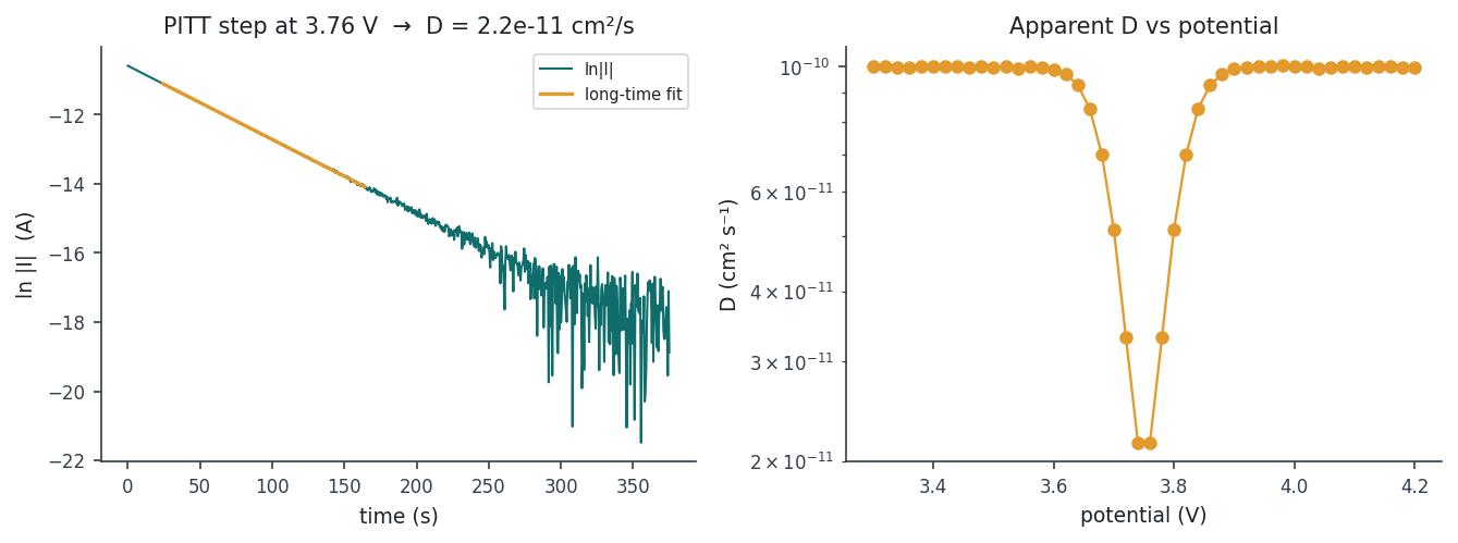
The same script gitt_pitt.py runs a full PITT pipeline too — it splits the staircase
into steps, fits the exponential tail of each for D, and plots D vs potential (its demo produced the
figure below; note the dip where a phase transition slows diffusion).
gitt_pitt.py.Electrode: mB = 1.5 mg, MB = 96 g mol⁻¹, density 4.8 g cm⁻³ → VM = 20 cm³ mol⁻¹, area S = 1.13 cm² (12 mm disk), pulse τ = 600 s. One step gives ΔEs = 8 mV and ΔEτ = 40 mV.
m_B·V_M / (M_B·S) = (1.5e-3 · 20)/(96 · 1.13) = 2.77e-4 cm

D = (4 / π·600) · (2.77e-4)² · (8/40)²  ≈  6.5 × 10⁻¹²  cm² s⁻¹
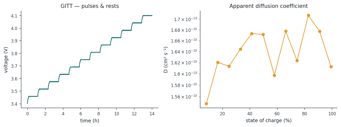
Do this for every step to get D vs SOC. The script gitt_pitt.py (in the
downloads) does it automatically from a data file — its demo produced the figure below.
gitt_pitt.py.- Report step size, duration, rest/cut-off criterion, temperature, direction, and how you got S or L (geometric vs BET vs particle size).
- Show a representative single step (E–√t for GITT, ln I–t for PITT) and plot D vs SOC for charge and discharge — never one headline number.
- The absolute D can be wrong by orders of magnitude (unknown true area / length); it is a relative measure. Call it apparent / chemical D.
- Phase-transition & conversion materials break the assumptions; GITT and PITT should agree if the physics is right.
References to read (start with 1–2): (1) Kim, Park, Hwang & Yoon, J. Electrochem. Sci. Technol. 13, 19 (2022) — open-access GITT review with full derivation; (2) Weppner & Huggins, J. Electrochem. Soc. 124, 1569 (1977) — the original GITT; (3) Li/Xie et al., Electrochim. Acta 51, 1039 (2005) — practical PITT; (4) Bard & Faulkner, Electrochemical Methods — Cottrell & diffusion basics; (5) the "spurious diffusion coefficient" papers (Electrochim. Acta 2002, 2004) — why the absolute numbers can mislead. Full list in the download.
Galvanostatic charge–discharge (GCD) — run, calculate & report
Constant-current cycling, the workhorse test: specific capacity, Coulombic efficiency, the voltage profile (energy, average voltage), capacity retention and rate capability, plus capacitance and ESR for capacitors — with how to choose the current/window and report multiple cycles and samples. Script, worked example, and references included.
GCD cycles the cell at constant current between two voltage cut-offs and records the voltage. It is the workhorse test — capacity, Coulombic efficiency, the voltage profile (energy, average voltage), cycle life, rate capability, and (for capacitors) capacitance and ESR. Most numbers in the battery reporting checklist come from here.
- Current — give C-rate and density (mA cm⁻²/g), and define what 1C means
- Voltage window (cut-offs); CC vs CC–CV — state the CV cut-off current
- Formation cycles — report a steady cycle, not the first
- Temperature, cycle count, cell format, and mass loading
Specific capacity   q  = I·Δt / (3.6·m)          [mAh/g]   (I[A], Δt[s], m[g])
Coulombic eff.      CE = Q_dis/Q_ch = Δt_dis/Δt_ch          [%]
Specific energy     E  = I·∫V dt /(3.6·m) [mWh/g];  V̄ = E/q
Retention           = Q_N / Q_1 × 100 %

Supercapacitor:  C = I / |dV/dt|  → C_spec = C/m [F/g]   (fit discharge slope, exclude IR)
                 ESR = ΔV_IR / (2·I) [Ω];   E = ½ C ΔV² ;   P = E/Δt_dis
Discharge at I = 1.5 mA for Δt = 1 h (3600 s) on m = 15 mg of active material:
q = I·Δt / (3.6·m) = (1.5e-3 · 3600) / (3.6 · 1.5e-2) = 100 mAh/g
If charge took 3600 s and discharge 3560 s:  CE = 3560/3600 = 98.9 %
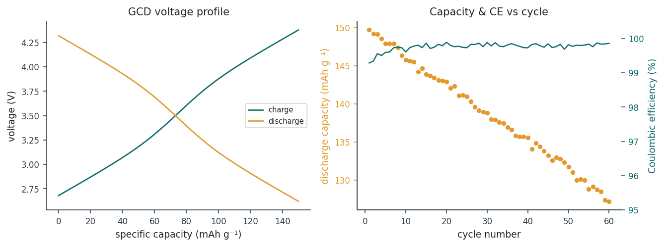
The script gcd.py (downloads) computes capacity, CE, energy,
retention, and supercap C/ESR from a data file — its demo produced the figure below.
gcd.py.- Cycles: report which cycle; plot capacity & CE vs cycle; show profiles at 1st/10th/Nth. Do not point-by-point average voltage profiles (smears plateaus) — show a representative one
- Samples: normalise (per g / cm²); report capacity, CE, retention as mean ± SD with n (≥3 cells); overlay capacity-vs-cycle, mean bold
- CE to enough sig-figs (99.92 %, not ~100 %); tiny losses compound over hundreds of cycles
- State the capacity basis; ultra-low loading inflates rate/cycling; CC–CV charge vs CC discharge lowers CE for protocol reasons
References to read (start with 1–2): (1) Stoller & Ruoff, "Best practical methods … supercapacitors," Energy Environ. Sci. 3, 1294 (2010); (2) the lab's Battery reporting checklist (same section) — what to disclose with any GCD result; (3) Bard & Faulkner, Electrochemical Methods — constant-current fundamentals; (4) BioLogic Application Note 51 — DC characterisation (capacity, energy, ESR, CE). Full list in the download.
Cyclic voltammetry (CV) — run, calculate & report
Sweep the potential and read the current: redox potentials, reversibility, whether the current is diffusion- or surface-controlled (b-value), the diffusion coefficient (Randles–Ševčík), the capacitive/diffusive split (Dunn), and capacitance — plus how to choose scan rates and windows and how to report multiple cycles and samples. Script, worked example, and references included.
CV sweeps the potential up and back at a constant scan rate v and records
the current. From the peaks and how they change with v you get redox potentials,
reversibility, the mechanism (diffusion vs surface), a diffusion coefficient, and capacitance.
Do the b-value check first — a "diffusion coefficient" only means something if the current is
actually diffusion-controlled.
- Reference electrode — state it; quote all potentials against it
- Window — inside electrolyte stability; only wide enough to capture the peaks
- Scan-rate range — cover ≥ a decade (e.g. 5–100 mV/s) so the slopes are well defined
- Cycles — report a stabilised cycle (3rd–5th), not the first (formation)
- iR compensation at high rates; 3-electrode cell; state area / active mass / temperature
Randles–Ševčík (reversible):  i_p = 2.69e5 · n^(3/2) · A · D^(1/2) · C · v^(1/2)
   → plot i_p vs √v ;  D = ( slope / (2.69e5 · n^(3/2) · A · C) )²

Reversibility:  ΔE_p = |E_pa − E_pc| ≈ 59/n mV ;  i_pa/i_pc ≈ 1 ;  E_p independent of v
b-value:        i_p = a·v^b  → log i_p vs log v ;  b≈0.5 diffusion, b≈1 surface/capacitive
Dunn split:     i(V) = k1·v + k2·√v   (capacitive + diffusion)
Capacitance:    C = (∮ i dV) / (2·v·ΔV) ;   C_specific = C / m
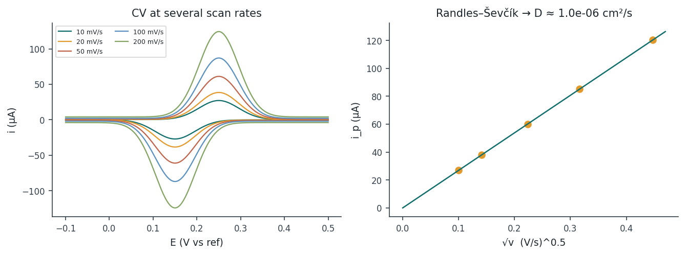
Redox couple: n = 1, A = 1 cm², C = 1 mM = 1×10⁻⁶ mol cm⁻³. The plot of i_p vs √v is linear with slope = 2.69×10⁻⁴ A/(V s⁻¹)^½. Then:
D = ( 2.69e-4 / (2.69e5 · 1 · 1 · 1e-6) )² = (1e-3)² = 1×10⁻⁶ cm² s⁻¹
The script cv.py (downloads) does this from your (v, i_p) data, plus the
b-value, Dunn split, and capacitance — its demo produced the figure below.
cv.py.- Cycles: report which cycle you show; use a stabilised one for quantitative reads; overlay cycle 1 → N to show activation
- Samples: fix window/rate set/reference/cycle; normalise current (mA cm⁻² or A g⁻¹); report E_p, i_p, D, C, b as mean ± SD with n; overlay CVs thin + representative bold
- b-value first — Randles–Ševčík is for diffusion-controlled reversible couples; capacitive current inflates i_p and it gives only an apparent D on porous electrodes
- iR drop distorts peaks at high v · geometric vs BET area shifts D · the first cycle is not steady state
References to read (start with 1–2): (1) Elgrishi et al., "A Practical Beginner's Guide to Cyclic Voltammetry," J. Chem. Educ. 95, 197 (2018) — the clearest intro; (2) Bard & Faulkner, Electrochemical Methods — CV theory & Randles–Ševčík; (3) Wang & Dunn et al., J. Phys. Chem. C 111, 14925 (2007) — the k1·v + k2·√v separation; (4) Brousse, Bélanger & Long, J. Electrochem. Soc. 162, A5185 (2015) — "To be or not to be pseudocapacitive?". Full list in the download.
EIS & DRT — measure, analyse, plot & report
Impedance spectroscopy and the distribution of relaxation times, kept simple: what each frequency region means, how to run and validate the measurement (Kramers–Kronig), how DRT deconvolutes overlapping processes, how to plot Nyquist/Bode/DRT correctly, and how to report replicates and multiple samples. Includes references for students.
EIS applies a tiny AC perturbation across frequency and measures
Z(ω) = Z′ − jZ″; because processes respond at different timescales, it separates them
by frequency. DRT is a model-free transform of the same data into a distribution
γ(τ) whose peaks resolve overlapping arcs — no equivalent circuit needed.
Both are only as good as the data: small amplitude, a stable cell, and a Kramers–Kronig check first.
- R_s / ohmic — high-frequency real-axis intercept (electrolyte + contacts + wiring)
- Film / SEI — high–mid frequency semicircle (if present)
- Charge transfer R_ct — mid-frequency semicircle; diameter = R_ct; use a CPE for a depressed arc
- Diffusion (Warburg) — low-frequency ~45° line
Run: small amplitude ~5–10 mV (stay linear), at an equilibrated OCV/SOC, wide range (~100 kHz–10 mHz, ≥6 pts/decade), state T and 2- vs 3-electrode. Validate with a Lin-KK test — structured low-frequency residuals usually mean the SOC drifted.
Read: R_s = high-f intercept; R_ct = semicircle diameter; apex frequency →
τ = 1/(2πf), C_dl = 1/(2π f R_ct). Equivalent-circuit fits must report the
circuit, values ± uncertainty, and χ² — and beware that many circuits fit the same data.
Z(ω) = R∞ + R_pol · ∫ γ(τ)/(1 + jωτ) dτ peak position = τ (f = 1/2πτ); peak area = its resistance
The inversion is ill-posed → Tikhonov regularisation with a parameter λ: too small = noisy, spurious peaks; too large = oversmoothed, merged peaks. Choose λ by the L-curve / GCV / discrepancy principle and report it. Use tools DRTtools (MATLAB) or pyDRTtools (Python) on KK-valid, low-noise data.
Assign peaks with evidence — watch how they move with temperature, SOC, or in a symmetric cell. A peak is a time constant, not automatically one physical step.
The script drt_pyDRTtools.py (downloads) is a real pipeline: load EIS → compute the
DRT with pyDRTtools, λ chosen by the L-curve → find the peaks (τ, f, R). The figure
below is a genuine DRT it produced — two RC arcs recovered as two peaks.
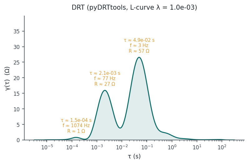
drt_pyDRTtools.py (pyDRTtools, L-curve λ). Peaks give the
process time constant τ (and f = 1/2πτ) and its resistance R (peak area).- Nyquist (−Z″ vs Z′) with equal (1:1) axes — unequal axes turn circles into ellipses and mislead. Mark frequency direction & decades
- Bode (|Z| and phase vs log f) alongside — Nyquist hides the frequency axis
- Overlay the fit + residuals; normalise to area (Ω·cm²) to compare samples
- DRT: γ(τ) vs log τ, label each peak, give λ + tool in the caption
Reading the spectrum below: Rs ≈ 8 Ω (high-frequency intercept). The DRT
resolves two processes — τ ≈ 2 ms (R ≈ 25 Ω) and τ ≈ 50 ms (R ≈ 60 Ω) — so
Rct,total ≈ 85 Ω. Each gives a capacitance C = τ/R: ≈ 80 µF and ≈ 830 µF.
The low-frequency 45° tail is diffusion (Warburg).
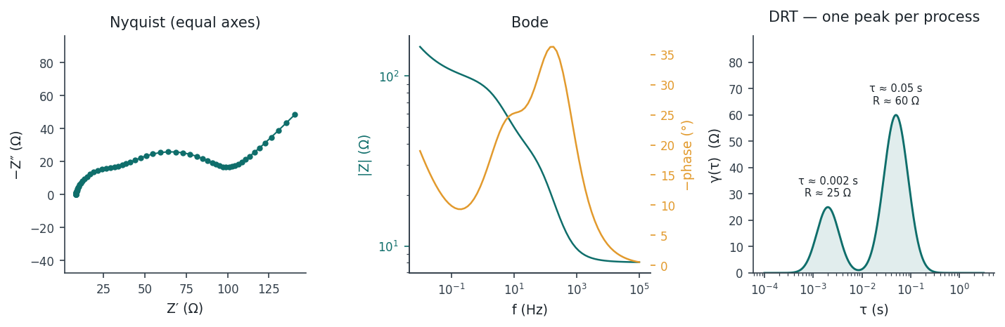
eis.py.
For real DRT on measured data use pyDRTtools and report λ.Quantitative EIS means fitting a circuit. The script eis_fit.py (downloads) fits
Rs–(R∥CPE)–…–Warburg circuits by complex least-squares and returns each value ± uncertainty
and χ². How to pick the circuit:
- Validate first (Lin-KK) — a bad spectrum can't be rescued by a circuit
- Let physics set the count: run the DRT — the number of peaks = number of R∥CPE arcs you need
- CPE, not ideal C, for depressed arcs; add a Warburg only if there's a low-frequency 45° tail
- Keep it simple (Occam): more elements always lower χ², but huge parameter uncertainties, or values that wander with the initial guess, mean over-fitting / a non-unique circuit
- Judge by the residuals (small & unstructured vs frequency), not χ² alone; tie every element to a physical process
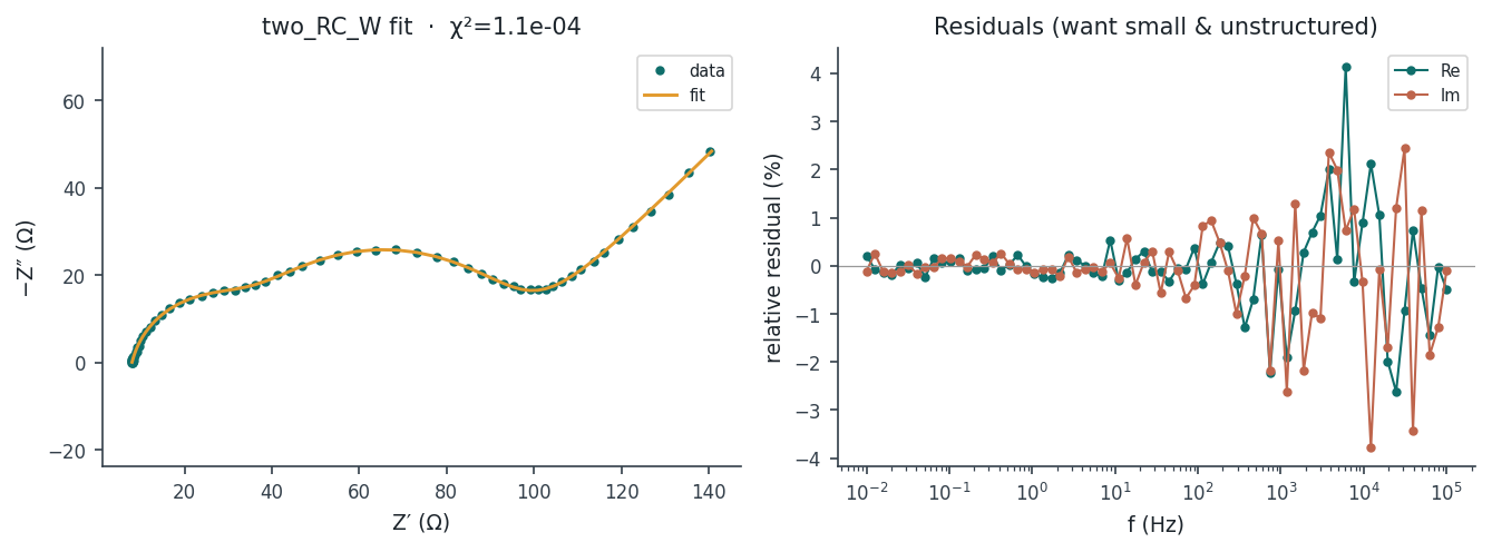
eis_fit.py. Small, unstructured residuals = a trustworthy fit; a good fit to the
wrong circuit is still wrong.- Fix SOC, T, amplitude, frequency range, equilibration — and, for DRT, the same λ and range — or spectra are not comparable
- Do not average raw spectra. Fit each cell, report parameters (R_s, R_ct, …) as mean ± SD with n; overlay all spectra thin + a representative one bold
- DRT: overlay γ(τ), report peak τ and area (R) as mean ± SD
- Account for excluded cells; state n, range, amplitude, T, SOC in every caption
References to read (start with 1–2): (1) Lasia, Electrochemical Impedance Spectroscopy and its Applications (Springer) — the teaching text; (2) Orazem & Tribollet, Electrochemical Impedance Spectroscopy (Wiley) — rigorous, incl. Kramers–Kronig; (3) Meddings et al., J. Power Sources 480, 228742 (2020) — EIS on real Li-ion cells; (4) Schönleber, Klotz & Ivers-Tiffée, Electrochim. Acta 131, 20 (2014) — the Lin-KK test; (5) Wan, Saccoccio, Chen & Ciucci, Electrochim. Acta 184, 483 (2015) — theory behind DRTtools/pyDRTtools. Full list and software links in the download.
Computational modelling
Molecular simulation and centrally managed cloud computing for defined mechanistic questions across the CTI chain.
Molecular simulation & cloud computing
We use molecular simulation when the question sits below the direct reach of an experiment: which ligands occupy the first coordination shell, how readily that shell reorganises, what crosses a polymer coating or nanopore, and what accumulates at an electrochemical interface.
A trajectory is not evidence until the model has passed a validation gate. Force-field provenance, thermodynamic checks, structural benchmarks, and comparison with experiment are part of the calculation—not optional additions after it.
What we can investigate
What the ion is wearing
- Radial distribution functions and coordination numbers
- First-shell solvent and anion populations
- Free ions, contact ion pairs, solvent-separated ion pairs, and larger aggregates
- Ligand-exchange and residence times
- Solvent activity and local hydrogen-bond structure
How it moves
- Mean-square displacement and self-diffusion coefficients
- Ion and solvent mobility
- Cluster transport and correlated motion
- Permeation through polymer coatings and nanopores
- Concentration, density, and composition profiles
What arrives and what is excluded
- Electrolyte organisation near metal, oxide, carbon, and polymer-coated surfaces
- Water and anion enrichment or depletion
- Ion accessibility and interfacial residence
- Transport across artificial interphases and protective coatings
- Molecular descriptors that can be compared with EIS/DRT, Raman, XAS, and electrochemical data
Systems the platform can support
The same workflow can be adapted to several systems studied in the group:
- aqueous, mixed-solvent, and additive-containing zinc electrolytes;
- zinc surfaces with polymer or artificial-interphase coatings;
- sodium-ion electrolytes and nanoconfined transport;
- organic and halogen-containing flow-battery electrolytes;
- porous-carbon electric-double-layer systems; and
- pseudocapacitive oxides, hydroxides, polymers, and framework materials.
The model and analysis must be designed for the scientific question. A force field that is adequate for bulk density is not automatically adequate for ion pairing, ligand exchange, or an interface.
Current computational stack
| Purpose | Tools |
|---|---|
| High-throughput classical molecular dynamics | GROMACS with NVIDIA CUDA acceleration |
| Materials and specialised interfacial molecular dynamics | LAMMPS with KOKKOS/CUDA |
| Initial molecular-box construction | Packmol |
| Structure preparation and workflow support | ASE and Python |
| Trajectory analysis | MDAnalysis, NumPy, SciPy, pandas |
| Figures and reports | Matplotlib and Jupyter |
| Compute infrastructure | On-demand RunPod GPU cloud with persistent project storage |
| Reproducibility | Version-controlled inputs, parameter provenance, validation records, and reusable analysis scripts |
Electronic-structure calculations and ab initio molecular dynamics using CP2K and Quantum ESPRESSO are planned extensions. They will be used only when the question requires explicit electronic structure, adsorption energetics, bond making or breaking, or interfacial charge redistribution.
How CTI guides the calculation
| CTI link | Representative computational descriptors |
|---|---|
| Coordination | RDF, coordination number, first-shell composition, free-solvent fraction, ion-pair population, residence time |
| Transport | Diffusion coefficient, cluster mobility, permeation, density profile, concentration profile |
| Interface | Interfacial composition, water/anion exclusion, adsorption geometry, local residence, access to active sites |
The aim is not simply to “run MD.” The aim is to identify a descriptor that connects molecular structure to transport and then to the measured interfacial response.
Validation before production
Every new chemical model must pass a documented validation stage before production trajectories are used as scientific evidence. Depending on the system, this may include:
- density and temperature stability;
- experimentally supported bond or ion–solvent distances;
- coordination number and first-shell geometry;
- radial distribution functions;
- diffusion coefficients;
- ion-pair or cluster populations;
- comparison with Raman, XAS, scattering, conductivity, viscosity, or electrochemical data; and
- confirmation that all numerical parameters have a traceable primary source.
Unvalidated parameters must not be mixed from unrelated force fields merely because the simulation runs without an error.
Current development
The first platform workflow is being developed for aqueous zinc electrolytes and the Zn | sulfonated polyimide | electrolyte interface. The workflow begins with validated bulk-electrolyte models, then progresses to polymer transport and the coated-zinc interface. The same infrastructure will subsequently support supercapacitor and pseudocapacitive systems.
Start with the research question
Computational resources are available to SKH Group members for approved research questions. Contact the PI before opening a cloud instance or starting a production calculation.
Please provide:
- the scientific question;
- the system and control to be compared;
- the electrolyte or material composition;
- the experimental observation or dataset that the model should explain;
- the CTI descriptor to be extracted; and
- an estimate of the number of conditions and independent replicas required.
Cloud instances, persistent storage, and production jobs are provisioned centrally. Do not create cloud resources or incur cloud charges independently without prior approval.
No previous MD experience is required to propose a project. Students will, however, be expected to understand the assumptions of the model, complete the benchmark and validation stage, and keep all inputs, scripts, and results under version control.
Start from the question, not the software.
“Which species replaces water in the first Zn²⁺ shell?” is a computational question.
“Run MD on this electrolyte” is not.
Figures & design
Colour, style, and templates for figures, posters, and slide decks.
Lab figure palette — Teal & Amber
The colour system for every figure we publish: papers, theses, posters, and slides. Drawing every figure from the same colours — in the same order and with the same meanings — is what makes our output recognisable, and it keeps figures readable for colour-blind readers and in greyscale, which most journals require. Start with the style guide, pin up the reference sheet, and apply it with the Python module or the AI prompt.
#0F6E6Bcontrol / baseline#E29A2Dthe effect of interest#BE654C3rd condition#5A91BE4th condition#83A4625th condition#995A906th condition#333F4Aaxes, ticks, text#DFC98Ffills / CI bands#1C242B#333F4A#66727C#B9C1C6#F3F0EBDrop labpalette.py beside your script, then one line applies the whole house style:
import labpalette as lp
lp.apply()                     # colours, fonts, 600 dpi
ax.plot(x, y, label="control") # cycles teal, amber, rust, ...
ax.imshow(Z, cmap=lp.cmap("teal"))
Open the AI prompt pack below, copy the block, and paste it into ChatGPT / Claude / Gemini before asking for a plot, diagram, or figure. It makes the AI use these exact colours and rules.
- teal = control/baseline, amber = the effect the figure is about.
- Use categorical colours in order; add marker shape or line style beyond 4 groups.
- Axes and text in graphite (#333F4A) — never pure black; gridlines in mist.
- Categorical for groups, ramps for continuous. Centre the diverging ramp on zero.
Full rationale, accessibility validation, and setup for R, Illustrator, LaTeX and CSS are in the style guide below.