4 Residence time and throughput
Problem 04 | Reactor Selection and Operating Conditions | Level 1: Guided problem
4.1 Problem Statement
Consider the parallel first-order reactions \(A\to D\) and \(A\to U\). Desired product \(D\) sells for 5 USD/kmol and byproduct \(U\) for 1 USD/kmol. Feed costs 1.2 USD/kmol. Fresh feed rate \(F\) is at most 100 kmol/h; at least 35 kmol/h of \(D\) must be produced. Unreacted feed has no recovery value. Constant density, constant temperature, and equal stoichiometric molar yields are assumed.
The synthetic kinetic functions are \[k_D=0.5a\exp[0.025(T-330)],\qquad k_U=0.08\exp[0.055(T-330)]\quad (\mathrm{h}^{-1}),\] where \(T\) is in K and \(a\) is a dimensionless activity factor. These functions are teaching data, not measured kinetics or a full Arrhenius model.
Heating costs \(0.006(T-320)\) USD per kmol of feed. The hourly equipment charge is 20 USD for a PFR or 10 USD for a CSTR. Available feed-equivalent holdup is \(F\tau\le250\) kmol. If inlet concentration is fixed at 1 kmol/m\(^3\), this corresponds to an equivalent volume limit of 250 m\(^3\). No pressure-drop, heat-transfer, or safety feasibility calculation is included.
Your task. Use a PFR at 330 K with activity \(a=1\). Choose residence time from 1, 2, 3, or 4 h and optimize feed rate and profit.
4.1.1 Before you code
Would maximizing conversion necessarily maximize profit when holdup is limited? Compare the throughput limits at residence times of 2 h and 4 h.
4.1.2 Deliverables
- Define decision variables, units, objective, and constraints. State which data and assumptions are fixed.
- Predict one feature of the solution and explain why it should occur.
- Build and solve a Pyomo model. Check balances and bounds independently.
- Interpret the result and investigate the follow-up question below. For an open-ended challenge, state and defend your chosen policy separately from the reference solution.
4.2 Model Formulation
For a mode \(j=(r_j,T_j,\tau_j)\), compute \(k=k_D+k_U\) and \[X_j=\begin{cases}1-e^{-k\tau_j}&r_j=\mathrm{PFR},\\ k\tau_j/(1+k\tau_j)&r_j=\mathrm{CSTR},\end{cases} \qquad y_{Dj}=X_j k_D/k,\quad y_{Uj}=X_j k_U/k.\] Let \(z_j\in\{0,1\}\) select a mode and \(f_j\ge0\) be its feed in kmol/h. Require \[\sum_jz_j=1,\quad f_j\le100z_j,\quad\sum_j\tau_j f_j\le250,\quad\sum_j y_{Dj}f_j\ge35.\] The profit for a fixed activity is \[\Pi=\sum_j\left[5y_{Dj}+y_{Uj}-1.2-0.006(T_j-320)\right]f_j-\sum_j K_{r_j}z_j.\] Although the kinetics are nonlinear in temperature and residence time, their values are constants for each listed mode. This gives a MILP that is globally optimal only over the stated finite menu, not over all continuous operating conditions.
Evaluate four modes and maximize \(\Pi\). Longer residence time raises conversion but reduces the throughput bound \(f_j\le250/\tau_j\). For a fixed mode the profit is linear in feed. Its feasible feed interval is \([35/y_{Dj},\min(100,250/\tau_j)]\). An empty interval means the mode cannot meet demand.
4.3 Pyomo Implementation
The code below is the model-building portion of models/reactors.py. The level argument selects this problem’s assumptions. Run the complete module from the source bundle to reproduce the solution, including its independent checks:
~/.venvs/optim/bin/python -m models.reactors 1"""Finite operating-menu reactor design with explicit kinetic assumptions."""
import math
import pyomo.environ as pyo
from models.common import value
FEED_MAX = 100.0 # kmol/h
VOLUME_MAX = 250.0 # flow-residence surrogate in kmol
DEMAND = 35.0 # kmol/h desired product
def yields(kind, temp, tau, activity=1.0):
kd = activity * 0.5 * math.exp(0.025 * (temp - 330))
ku = 0.08 * math.exp(0.055 * (temp - 330))
k = kd + ku
conversion = 1 - math.exp(-k * tau) if kind == "PFR" else k * tau / (1 + k * tau)
return conversion * kd / k, conversion * ku / k
def menu(level):
return [
(kind, t, tau)
for kind in (["PFR"] if level == 1 else ["PFR", "CSTR"])
for t in ([330] if level == 1 else [320, 330, 340, 350])
for tau in ([1, 2, 3, 4] if level == 1 else [0.5, 1, 2, 3, 4])
]
def build(level):
modes = menu(level)
states = (
{"nominal": 1.0} if level < 3 else {"low_activity": 0.8, "high_activity": 1.2}
)
m = pyo.ConcreteModel(name="Reactor operating menu")
m.J = pyo.RangeSet(0, len(modes) - 1)
m.S = pyo.Set(initialize=list(states))
m.z = pyo.Var(m.J, domain=pyo.Binary)
m.f = pyo.Var(m.J, domain=pyo.NonNegativeReals)
m.one = pyo.Constraint(expr=sum(m.z[j] for j in m.J) == 1)
m.bound = pyo.Constraint(m.J, rule=lambda m, j: m.f[j] <= FEED_MAX * m.z[j])
m.holdup = pyo.Constraint(expr=sum(modes[j][2] * m.f[j] for j in m.J) <= VOLUME_MAX)
yd = {(s, j): yields(*modes[j], states[s])[0] for s in states for j in m.J}
yu = {(s, j): yields(*modes[j], states[s])[1] for s in states for j in m.J}
m.product = pyo.Constraint(
m.S, rule=lambda m, s: sum(yd[s, j] * m.f[j] for j in m.J) >= DEMAND
)
def profit(m, s):
return sum(
(5 * yd[s, j] + yu[s, j] - 1.2 - 0.006 * (modes[j][1] - 320)) * m.f[j]
- (20 if modes[j][0] == "PFR" else 10) * m.z[j]
for j in m.J
)
m.profit = pyo.Expression(m.S, rule=profit)
m.eta = pyo.Var(bounds=(-1000, 1000))
m.floor = pyo.Constraint(m.S, rule=lambda m, s: m.eta <= m.profit[s])
m.obj = pyo.Objective(expr=m.eta, sense=pyo.maximize)
m._modes = modes
m._states = states
return mThe common solve function calls appsi_highs, checks optimal termination before loading a solution, and checks constraint residuals, bounds, and integer domains. After building the model, use:
from models.common import solve
m = solve(build(1))
4.4 Optimal Solution
The reference objective is 180.6261 USD/h. This value is optimal for the explicitly stated model and data.
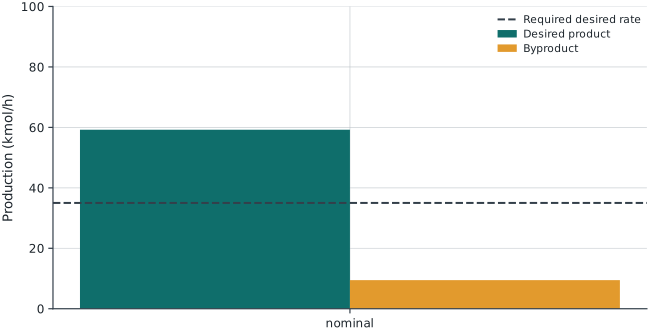
| State | Desired (kmol/h) | Undesired (kmol/h) | Profit (USD/h) |
|---|---|---|---|
| nominal | 59.2299 | 9.4768 | 180.6261 |
| Quantity | Value |
|---|---|
| Reactor | PFR |
| Temperature (K) | 330.0000 |
| Residence time (h) | 3.0000 |
| Feed (kmol/h) | 83.3333 |
| Holdup (kmol) | 250.0000 |
4.4.1 Check your solution
Enumerate the four modes independently and calculate the optimal endpoint of each feasible feed interval. Confirm \(D+U+\text{unreacted A}=F\).
The automated residual, bound, and integrality audit passed with a maximum violation of 2.84e-14 in model units. Domain-specific checks passed. Model units differ across equations, so this numerical audit does not replace dimensional analysis.
4.5 Brief Discussion
The selected PFR operates at 330 K and 3.0 h with feed 83.333 kmol/h. The objective is 180.626 USD/h. The feed-holdup tradeoff, product selectivity, and operating cost are included in this choice. Enumerating the same menu independently reproduces the optimum. Refining the menu is a different model, not a stronger claim about this result.
4.5.1 Extension to investigate
Change the desired-product price to 4 USD/kmol. Explain why the preferred residence time may or may not change.