7 Dispatch through existing exchangers
Problem 07 | Heat Recovery Network Design | Level 1: Guided problem
7.1 Problem Statement
Two fixed-temperature heat sources provide 120 kW at 180 °C (H1) and 80 kW at 110 °C (H2). Heat users require 100 kW at 150 °C (C1) and 100 kW at 80 °C (C2). A minimum approach of 20 °C allows H1-C1, H1-C2, and H2-C2; H2-C1 is forbidden. These are isothermal source/sink surrogates, not sensible-heat streams with temperature profiles.
| Match | Maximum recovered heat (kW) | Daily installation charge (USD/d) |
|---|---|---|
| H1-C1 | 100 | 25 |
| H1-C2 | 90 | 20 |
| H2-C2 | 70 | 18 |
Hot utility costs 1 USD/(kW d); cold utility costs 0.15 USD/(kW d). These coefficients already convert a constant daily heat rate to a daily cost. Do not multiply by 24 again. Utilities are available at suitable temperatures without capacity limits. All unused source heat must be rejected.
Your task. Assume all three exchangers are already installed and their installation charges are sunk. Minimize daily utility cost.
7.1.1 Before you code
Total source heat equals total demand. Does that guarantee zero hot utility when match capacities and temperature feasibility are respected?
7.1.2 Deliverables
- Define decision variables, units, objective, and constraints. State which data and assumptions are fixed.
- Predict one feature of the solution and explain why it should occur.
- Build and solve a Pyomo model. Check balances and bounds independently.
- Interpret the result and investigate the follow-up question below. For an open-ended challenge, state and defend your chosen policy separately from the reference solution.
7.2 Model Formulation
Let \(q_{hcs}\ge0\) be recovered heat on an allowed match, \(u_{cs}\ge0\) hot utility, and \(v_{hs}\ge0\) rejected heat, all in kW. Let \(z_{hc}\in\{0,1\}\) select an exchanger. For each operating state \(s\), \[\sum_c q_{hcs}+v_{hs}=H_h,\qquad \sum_h q_{hcs}+u_{cs}=D_{cs},\qquad q_{hcs}\le\overline Q_{hc}z_{hc}.\] Only allowed matches appear in the sums. The first balance accounts for surplus heat, while the second prevents counting recovered heat twice. Installation charges are daily equivalents of ownership costs, not one-time capital expenses.
Fix every \(z_{hc}=1\) and solve the LP \[\min C=\sum_c u_c+0.15\sum_h v_h.\] The network has 200 kW on each side, but the H2-C2 limit prevents full recovery. Simultaneous hot and cold utility is therefore possible even with equal aggregate supply and demand.
7.3 Pyomo Implementation
The code below is the model-building portion of models/heat.py. The level argument selects this problem’s assumptions. Run the complete module from the source bundle to reproduce the solution, including its independent checks:
~/.venvs/optim/bin/python -m models.heat 1"""Heat recovery between fixed-temperature utility-like streams."""
import pyomo.environ as pyo
from models.common import value
HOT = {"H1": 120, "H2": 80} # kW available
ARCS = [("H1", "C1"), ("H1", "C2"), ("H2", "C2")]
CAP = {("H1", "C1"): 100, ("H1", "C2"): 90, ("H2", "C2"): 70}
FIXED = {("H1", "C1"): 25, ("H1", "C2"): 20, ("H2", "C2"): 18} # USD/d
def build(level):
states = (
{"normal": (100, 100, 1.0, 1.0)}
if level < 3
else {"low": (100, 80, 1.0, 0.5), "high": (100, 130, 2.0, 0.5)}
)
m = pyo.ConcreteModel(name="Fixed-temperature heat recovery")
m.A = pyo.Set(initialize=ARCS, dimen=2)
m.H = pyo.Set(initialize=list(HOT))
m.C = pyo.Set(initialize=["C1", "C2"])
m.S = pyo.Set(initialize=list(states))
m.z = pyo.Var(m.A, domain=pyo.Binary)
if level == 1:
for a in m.A:
m.z[a].fix(1)
m.q = pyo.Var(m.S, m.A, domain=pyo.NonNegativeReals)
m.hu = pyo.Var(m.S, m.C, domain=pyo.NonNegativeReals)
m.cu = pyo.Var(m.S, m.H, domain=pyo.NonNegativeReals)
m.hot = pyo.Constraint(
m.S,
m.H,
rule=lambda m, s, h: (
sum(m.q[s, i, j] for i, j in m.A if i == h) + m.cu[s, h] == HOT[h]
),
)
m.cold = pyo.Constraint(
m.S,
m.C,
rule=lambda m, s, c: (
sum(m.q[s, i, j] for i, j in m.A if j == c) + m.hu[s, c]
== states[s][0 if c == "C1" else 1]
),
)
m.cap = pyo.Constraint(
m.S, m.A, rule=lambda m, s, h, c: m.q[s, h, c] <= CAP[h, c] * m.z[h, c]
)
if level == 3:
m.budget = pyo.Constraint(expr=sum(FIXED[a] * m.z[a] for a in m.A) <= 45)
fixed = 0 if level == 1 else sum(FIXED[a] * m.z[a] for a in m.A)
m.obj = pyo.Objective(
expr=fixed
+ sum(
states[s][3]
* (
states[s][2] * sum(m.hu[s, c] for c in m.C)
+ 0.15 * sum(m.cu[s, h] for h in m.H)
)
for s in m.S
)
)
m._states = states
return mThe common solve function calls appsi_highs, checks optimal termination before loading a solution, and checks constraint residuals, bounds, and integer domains. After building the model, use:
from models.common import solve
m = solve(build(1))
7.4 Optimal Solution
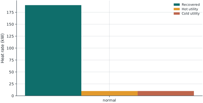
The reference objective is 11.5000 USD/d. This value is optimal for the explicitly stated model and data.
| State | Match | Installed | Heat (kW) |
|---|---|---|---|
| normal | H1 to C1 | 1 | 100.0000 |
| normal | H1 to C2 | 1 | 20.0000 |
| normal | H2 to C2 | 1 | 70.0000 |
| Quantity | Value |
|---|---|
| normal: hot utility (kW) | 10.0000 |
| normal: cold utility (kW) | 10.0000 |
7.4.1 Check your solution
Calculate recovered heat and both utility totals. Confirm \(\text{hot utility}-\text{cold utility}=\text{total demand}-\text{total source heat}\).
The automated residual, bound, and integrality audit passed with a maximum violation of 0.00e+00 in model units. Domain-specific checks passed. Model units differ across equations, so this numerical audit does not replace dimensional analysis.
7.5 Brief Discussion
The objective is 11.50 USD/d. The existing system still needs 10 kW of hot utility and rejects 10 kW because the match limits prevent full recovery. For a physical exchanger network with varying stream temperatures, stagewise temperature balances and minimum approaches would need to replace this fixed-temperature representation.
7.5.1 Extension to investigate
Increase the H2-C2 capacity from 70 to 80 kW. Predict the change in both utilities and daily cost before solving.