18 Selecting treatment under composition uncertainty
Problem 18 | Wastewater Treatment and Reuse | Level 3: Open-ended challenge
18.1 Problem Statement
Two independent wastewater sources supply S1 = 60 m\(^3\)/h at 40 mg/L and S2 = 50 m\(^3\)/h at 120 mg/L of one contaminant. Users U1 and U2 need 50 and 40 m\(^3\)/h, with maximum inlet concentrations of 30 and 60 mg/L. Freshwater contains no contaminant and costs 1 USD/m\(^3\). Unused source water is discharged at 0.10 USD/m\(^3\). User outlet streams are outside the model boundary; this is a one-pass reuse allocation.
| Treatment | Removal fraction | Capacity (m3/h) | Variable cost (USD/m3) | Hourly ownership charge (USD/h) |
|---|---|---|---|---|
| Moderate | 0.75 | 40 | 0.25 | 3 |
| Advanced | 0.95 | 80 | 0.45 | 12 |
Treatment conserves water volume and transfers removed contaminant to a separate captured-residue stream. Residue handling is included in the assumed treatment cost. Each source remains segregated through treatment, or equivalently uses source-specific modules with a shared total hydraulic capacity. Fixed removal fractions do not depend on loading. These assumptions avoid a common mixed treatment inlet with an unknown concentration.
Your task. Choose at most one new treatment option, or none. Source concentrations can independently rise to 60 mg/L for S1 and 160 mg/L for S2. Require all user quality limits to hold throughout these intervals, using one fixed allocation. Minimize the deterministic cost including the selected hourly ownership charge. Explain when the segregated treatment assumption would be defensible.
18.1.1 Before you code
Which concentrations create the worst load? What nonlinear term appears if an intermediate mixed pool has both unknown flow and unknown concentration?
18.1.2 Deliverables
- Define decision variables, units, objective, and constraints. State which data and assumptions are fixed.
- Predict one feature of the solution and explain why it should occur.
- Build and solve a Pyomo model. Check balances and bounds independently.
- Interpret the result and investigate the follow-up question below. For an open-ended challenge, state and defend your chosen policy separately from the reference solution.
18.2 Model Formulation
Let \(x_{ij}\ge0\) be direct reuse, \(y_{ijk}\ge0\) treated reuse through technology \(k\), \(f_j\ge0\) freshwater, and \(d_i\ge0\) discharge, all in m\(^3\)/h. A binary \(z_k\) selects a treatment option when required. With source supply \(S_i\), user demand \(D_j\), source concentration \(c_i\), user limit \(L_j\), and removal \(r_k\), \[\sum_j\left(x_{ij}+\sum_ky_{ijk}\right)+d_i=S_i,\] \[\sum_i\left(x_{ij}+\sum_ky_{ijk}\right)+f_j=D_j,\] \[\sum_i c_i\left[x_{ij}+\sum_k(1-r_k)y_{ijk}\right]\le L_jD_j,\] \[\sum_{i,j}y_{ijk}\le\overline Q_k z_k.\] Concentration-times-flow products have units mg/L times m\(^3\)/h. Multiplying every term by 1000 gives mg/h, so the common factor cancels in the quality inequality. Concentrations are fixed input coefficients, which keeps this formulation linear.
Use the upper concentrations in every quality inequality, since all flows and residual fractions are nonnegative. Require \(\sum_kz_k\le1\) and minimize \[C=\sum_jf_j+0.10\sum_id_i+\sum_{i,j,k}v_ky_{ijk}+\sum_kK_kz_k.\] This is a robust MILP for fixed-quality, segregated treatment paths. In a general pooling model, a pool concentration \(c_P\) and outgoing flow \(q_{Pj}\) are both variables, producing the bilinear load \(c_Pq_{Pj}\). The present solution is not a global solution to that unrestricted nonlinear pooling problem. A separate nonlinear model and suitable solver would be required for it.
18.3 Pyomo Implementation
The code below is the model-building portion of models/water.py. The level argument selects this problem’s assumptions. Run the complete module from the source bundle to reproduce the solution, including its independent checks:
~/.venvs/optim/bin/python -m models.water 3"""Segregated wastewater reuse with fixed-quality source streams."""
import pyomo.environ as pyo
from models.common import value
SUPPLY = {"S1": 60, "S2": 50} # m3/h
NOMINAL = {"S1": 40, "S2": 120} # mg/L
HIGH = {"S1": 60, "S2": 160}
DEMAND = {"U1": 50, "U2": 40} # m3/h
LIMIT = {"U1": 30, "U2": 60} # mg/L
TECH = {"moderate": (0.75, 40, 0.25, 3), "advanced": (0.95, 80, 0.45, 12)}
# removal fraction, hydraulic capacity m3/h, variable USD/m3, fixed USD/h
def build(level):
conc = HIGH if level == 3 else NOMINAL
techs = [] if level == 1 else ["moderate"] if level == 2 else list(TECH)
m = pyo.ConcreteModel(name="Segregated water reuse")
m.I = pyo.Set(initialize=list(SUPPLY))
m.J = pyo.Set(initialize=list(DEMAND))
m.K = pyo.Set(initialize=techs)
m.x = pyo.Var(m.I, m.J, domain=pyo.NonNegativeReals)
m.y = pyo.Var(m.I, m.J, m.K, domain=pyo.NonNegativeReals)
m.f = pyo.Var(m.J, domain=pyo.NonNegativeReals)
m.d = pyo.Var(m.I, domain=pyo.NonNegativeReals)
m.z = pyo.Var(m.K, domain=pyo.Binary)
if level == 2:
m.z["moderate"].fix(1)
if level == 3:
m.choose = pyo.Constraint(expr=sum(m.z[k] for k in m.K) <= 1)
m.source = pyo.Constraint(
m.I,
rule=lambda m, i: (
sum(m.x[i, j] + sum(m.y[i, j, k] for k in m.K) for j in m.J) + m.d[i]
== SUPPLY[i]
),
)
m.sink = pyo.Constraint(
m.J,
rule=lambda m, j: (
sum(m.x[i, j] + sum(m.y[i, j, k] for k in m.K) for i in m.I) + m.f[j]
== DEMAND[j]
),
)
m.quality = pyo.Constraint(
m.J,
rule=lambda m, j: (
sum(
conc[i]
* (m.x[i, j] + sum((1 - TECH[k][0]) * m.y[i, j, k] for k in m.K))
for i in m.I
)
<= LIMIT[j] * DEMAND[j]
),
)
m.cap = pyo.Constraint(
m.K,
rule=lambda m, k: (
sum(m.y[i, j, k] for i in m.I for j in m.J) <= TECH[k][1] * m.z[k]
),
)
m.obj = pyo.Objective(
expr=sum(m.f[j] for j in m.J)
+ 0.1 * sum(m.d[i] for i in m.I)
+ sum(TECH[k][2] * m.y[i, j, k] for i in m.I for j in m.J for k in m.K)
+ (sum(TECH[k][3] * m.z[k] for k in m.K) if level == 3 else 0)
)
m._conc = conc
return mThe common solve function calls appsi_highs, checks optimal termination before loading a solution, and checks constraint residuals, bounds, and integer domains. After building the model, use:
from models.common import solve
m = solve(build(3))
18.4 Optimal Solution
The reference objective is 20.8235 USD/h. This value is optimal for the explicitly stated model and data.
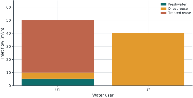
| User | Fresh (m3/h) | Direct reuse (m3/h) | Treated reuse (m3/h) | Concentration (mg/L) |
|---|---|---|---|---|
| U1 | 5.2941 | 4.7059 | 40.0000 | 30.0000 |
| U2 | 0.0000 | 40.0000 | 0.0000 | 60.0000 |
| Quantity | Value |
|---|---|
| Freshwater (m3/h) | 5.2941 |
| Disposal (m3/h) | 25.2941 |
| Technology | moderate |
18.4.1 Check your solution
Check the worst-case water and contaminant balances. Fix each of the three choices (none, moderate, advanced), solve its allocation LP, and compare the feasible costs.
The automated residual, bound, and integrality audit passed with a maximum violation of 0.00e+00 in model units. Domain-specific checks passed. Model units differ across equations, so this numerical audit does not replace dimensional analysis.
18.5 Brief Discussion
The solution uses 5.294 m3/h of freshwater and discharges 25.294 m3/h, at 20.824 USD/h. Treatment choice: moderate. Contaminant removed by treatment must leave in the captured-residue stream. Fixed removal and segregated paths are substantive process assumptions, not just numerical conveniences.
18.5.1 Extension to investigate
Propose an unrestricted pool formulation with flow and concentration variables. Identify its bilinear equations and explain what additional measurements or bounds would be required before solving.