14 Choosing tank capacity
Problem 14 | Hydrogen Production and Storage | Level 2: Model extension
14.1 Problem Statement
An electrolyzer operates over six four-hour periods, representing one day. Electricity use is constant at 0.05 MWh/kg of hydrogen. Power is limited to 4 MW. Initial hydrogen inventory is 50 kg, and final inventory must also be 50 kg. Storage has no leakage and no charging-rate restriction. Production and withdrawal rates are each uniform within a period. Inventory therefore varies linearly between period boundaries.
| Period | Electricity price (USD/MWh) | Hydrogen demand (kg/period) |
|---|---|---|
| 1 | 30 | 120 |
| 2 | 25 | 150 |
| 3 | 80 | 180 |
| 4 | 100 | 220 |
| 5 | 45 | 180 |
| 6 | 35 | 140 |
Capacity is enforced at every period boundary, including the 50 kg initial stock. Under the uniform-rate assumption, this also bounds inventory throughout each period. If deliveries are discrete or rates vary within a period, an additional inventory profile or shorter time steps is necessary for physical sizing. A daily capacity charge of 0.15 USD/(kg d) is used where investment is optimized. It is an assumed daily equivalent, not a full capital-cost model.
Your task. Choose \(50\le K\le500\) kg and minimize electricity cost plus the daily capacity charge. Compare with the 150 kg tank, charging that fixed tank the same daily capacity rate for a fair total-cost comparison.
14.1.1 Before you code
Can additional storage change total daily electricity use in this constant-efficiency model? If not, where do the savings come from?
14.1.2 Deliverables
- Define decision variables, units, objective, and constraints. State which data and assumptions are fixed.
- Predict one feature of the solution and explain why it should occur.
- Build and solve a Pyomo model. Check balances and bounds independently.
- Interpret the result and investigate the follow-up question below. For an open-ended challenge, state and defend your chosen policy separately from the reference solution.
14.2 Model Formulation
Let \(P_{st}\) be power in MW, \(I_{st}\) end inventory in kg, and \(K\) capacity in kg. With \(\Delta t=4\) h and \(e=0.05\) MWh/kg, \[I_{st}=I_{s,t-1}+\frac{\Delta t}{e}P_{st}-D_{st},\qquad 0\le P_{st}\le4,\quad0\le I_{st}\le K.\] Use \(I_{s0}=50\) before the first period and \(I_{s6}=50\) at the end. Total production must equal total demand. The electricity cost is \(\sum_t c_t\Delta t P_{st}\) USD/d. Omitting \(\Delta t\) would understate cost by a factor of four.
Solve \[\min C=0.15K+\sum_t c_t\Delta tP_t.\] The lower bound of 50 kg accommodates initial and final stock. This LP values the timing of production, not a change in thermodynamic efficiency. The comparison with Problem 13 must add \(0.15(150)\) USD/d to its electricity-only objective.
14.3 Pyomo Implementation
The code below is the model-building portion of models/hydrogen.py. The level argument selects this problem’s assumptions. Run the complete module from the source bundle to reproduce the solution, including its independent checks:
~/.venvs/optim/bin/python -m models.hydrogen 2"""Daily hydrogen dispatch, tank design, and scenario-dependent operation."""
import pyomo.environ as pyo
from models.common import value
PRICE = [30, 25, 80, 100, 45, 35] # USD/MWh
DEMAND = [120, 150, 180, 220, 180, 140] # kg per four-hour period
DT = 4 # h
SPECIFIC_ENERGY = 0.05 # MWh/kg
TANK_CHARGE = 0.15 # USD/(kg capacity d)
def build(level):
states = (
{"nominal": (1, 1)} if level < 3 else {"low": (0.9, 0.5), "high": (1.15, 0.5)}
)
m = pyo.ConcreteModel(name="Hydrogen production and storage")
m.S = pyo.Set(initialize=list(states))
m.T = pyo.RangeSet(0, 5)
m.k = pyo.Var(bounds=(50, 500))
if level == 1:
m.k.fix(150)
m.power = pyo.Var(m.S, m.T, bounds=(0, 4))
m.stock = pyo.Var(m.S, m.T, domain=pyo.NonNegativeReals)
m.balance = pyo.Constraint(
m.S,
m.T,
rule=lambda m, s, t: (
m.stock[s, t]
== (50 if t == 0 else m.stock[s, t - 1])
+ DT * m.power[s, t] / SPECIFIC_ENERGY
- DEMAND[t] * states[s][0]
),
)
m.capacity = pyo.Constraint(m.S, m.T, rule=lambda m, s, t: m.stock[s, t] <= m.k)
m.terminal = pyo.Constraint(m.S, rule=lambda m, s: m.stock[s, 5] == 50)
if level == 3:
m.on = pyo.Var(m.S, m.T, domain=pyo.Binary)
m.start = pyo.Var(m.S, m.T, domain=pyo.Binary)
m.upper = pyo.Constraint(
m.S, m.T, rule=lambda m, s, t: m.power[s, t] <= 4 * m.on[s, t]
)
m.lower = pyo.Constraint(
m.S, m.T, rule=lambda m, s, t: m.power[s, t] >= m.on[s, t]
)
m.startup = pyo.Constraint(
m.S,
m.T,
rule=lambda m, s, t: (
m.start[s, t] >= m.on[s, t] - (0 if t == 0 else m.on[s, t - 1])
),
)
fixed = 0 if level == 1 else TANK_CHARGE * m.k
m.obj = pyo.Objective(
expr=fixed
+ sum(
states[s][1]
* sum(
DT * PRICE[t] * m.power[s, t]
+ (10 * m.start[s, t] if level == 3 else 0)
for t in m.T
)
for s in m.S
)
)
m._states = states
return mThe common solve function calls appsi_highs, checks optimal termination before loading a solution, and checks constraint residuals, bounds, and integer domains. After building the model, use:
from models.common import solve
m = solve(build(2))
14.4 Optimal Solution
The reference objective is 1,635.5000 USD/d. This value is optimal for the explicitly stated model and data.
| State | Period | Power (MW) | Demand (kg) | End stock (kg) |
|---|---|---|---|---|
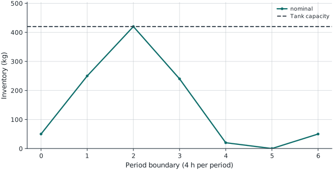
| nominal | 1 | 4.0000 | 120 | 250.0000 |
| nominal | 2 | 4.0000 | 150 | 420.0000 |
| nominal | 3 | 0.0000 | 180 | 240.0000 |
| nominal | 4 | 0.0000 | 220 | 20.0000 |
| nominal | 5 | 2.0000 | 180 | 0.0000 |
| nominal | 6 | 2.3750 | 140 | 50.0000 |
| Quantity | Value |
|---|---|
| Tank capacity (kg) | 420.0000 |
| Expected electricity (MWh/d) | 49.5000 |
14.4.1 Check your solution
Check the chosen tank is large enough for every reported end stock. Re-solve with fixed capacity values and verify that electricity savings eventually cease as capacity grows.
The automated residual, bound, and integrality audit passed with a maximum violation of 0.00e+00 in model units. Domain-specific checks passed. Model units differ across equations, so this numerical audit does not replace dimensional analysis.
14.4.2 Fixed-capacity experiment
| capacity_kg | total_cost | electricity_cost |
|---|---|---|
| 50.0000 | 2670.0000 | 2662.5000 |
| 100.0000 | 2490.0000 | 2475.0000 |
| 150.0000 | 2310.0000 | 2287.5000 |
| 200.0000 | 2137.5000 | 2107.5000 |
| 300.0000 | 1882.5000 | 1837.5000 |
| 400.0000 | 1647.5000 | 1587.5000 |
| 420.0000 | 1635.5000 | 1572.5000 |
| 450.0000 | 1640.0000 | 1572.5000 |
| 500.0000 | 1647.5000 | 1572.5000 |
14.5 Brief Discussion
The selected tank is 420.0 kg. Total daily cost is 1635.50 USD versus 2310.00 USD for the fixed 150 kg tank with the same ownership charge, saving 674.50 USD/d (29.20%). This is a daily-equivalent planning result under uniform within-period flows.
14.5.1 Extension to investigate
Estimate the break-even daily capacity charge for increasing the tank beyond 150 kg. Describe how finer time resolution might alter the design.