3 Production Planning with Scheduled Maintenance
Based on Factory planning 1, Section 12.3 of Williams (2013). New three-product, three-month teaching instance for a specialty chemical plant; replaces the seven-product numerical instance. The results below solve the stated instance and are not presented as the numerical answer to an unmodified textbook problem.
3.1 Problem Statement
A specialty chemical plant produces grades A, B, and C over three months. Processing contribution margins (before holding cost) are 8, 10, and 12 thousand USD/t. Reactor hours per tonne are 2, 3, and 4; finishing hours are 3, 2, and 2. Monthly reactor availability is 120, 80, 120 h and finishing availability is 100, 100, 80 h, after scheduled maintenance. Sales limits (A,B,C) are (20,15,10), (15,20,15), (20,15,20) t. Initial stocks are zero, final stocks must be 5 t per grade, and month-end storage is limited to 15 t per grade. Holding cost is 0.5 thousand USD/t at every month-end, including month 3. Choose production, sales, and inventories to maximize total contribution. Final stock has no sale or salvage credit in this horizon. There is no requirement to satisfy all sales opportunities.
3.1.1 Product data
| Grade | Margin (1000 USD/t) | Reactor (h/t) | Finishing (h/t) |
|---|---|---|---|
| A | 8 | 2 | 3 |
| B | 10 | 3 | 2 |
| C | 12 | 4 | 2 |
3.1.2 Monthly data
| Month | A sales cap (t) | B sales cap (t) | C sales cap (t) | Reactor (h) | Finishing (h) |
|---|---|---|---|---|---|
| 1 | 20 | 15 | 10 | 120 | 100 |
| 2 | 15 | 20 | 15 | 80 | 100 |
| 3 | 20 | 15 | 20 | 120 | 80 |
3.2 Model Formulation
Let \(x_{it},z_{it},s_{it}\ge0\) be production, sales, and closing stock (t). Parameters are contribution \(p_i\), holding charge \(h\), processing hours \(a_{ri}\), capacity \(C_{rt}\), and sales limit \(D_{it}\).
\[\max\sum_{it}(p_i z_{it}-h s_{it}),\qquad s_{i,t-1}+x_{it}=z_{it}+s_{it}.\]
\[\sum_i a_{ri}x_{it}\le C_{rt},\quad z_{it}\le D_{it},\quad0\le s_{it}\le15,\quad s_{i0}=0,\ s_{i3}=5.\]
Production consumes capacity; sales generate contribution. These are distinct variables because inventory can connect months. Capacity is supplied after maintenance, so maintenance decisions are not optimized in this LP.
All decision variables and units refer to the problem statement above. Continuous variables are nonnegative unless explicitly stated otherwise; binary and integer domains are specified in the equations and code.
3.3 Pyomo Implementation
The following Python implementation uses Pyomo and HiGHS. Run from the workbook root so that the models package and shared helpers are importable. The shared solver and audit functions check optimal termination before loading values, then verify every active constraint, variable bound, and integer domain. Any imported earlier-chapter model supplies the data and balances already explained there.
The full source is problem03.py. To solve and print this problem independently:
~/.venvs/optim/bin/python -m models.common 3import pyomo.environ as pyo
from models.common import frame
PRODUCTS = ["A", "B", "C"]
MARGIN = {"A": 8, "B": 10, "C": 12}
HOURS = {"reactor": [2, 3, 4], "finishing": [3, 2, 2]}
CAPACITY = {"reactor": [120, 80, 120], "finishing": [100, 100, 80]}
DEMAND = [[20, 15, 10], [15, 20, 15], [20, 15, 20]]
def build():
m = pyo.ConcreteModel()
m.I = pyo.Set(initialize=PRODUCTS)
m.T = pyo.RangeSet(0, 2)
m.make = pyo.Var(m.I, m.T, domain=pyo.NonNegativeReals)
m.sell = pyo.Var(m.I, m.T, domain=pyo.NonNegativeReals)
m.stock = pyo.Var(m.I, m.T, bounds=(0, 15))
m.balance = pyo.Constraint(
m.I,
m.T,
rule=lambda m, i, t: (
(m.stock[i, t - 1] if t else 0) + m.make[i, t]
== m.sell[i, t] + m.stock[i, t]
),
)
m.demand = pyo.Constraint(
m.I, m.T, rule=lambda m, i, t: m.sell[i, t] <= DEMAND[t][PRODUCTS.index(i)]
)
m.final = pyo.Constraint(m.I, rule=lambda m, i: m.stock[i, 2] == 5)
m.capacity = pyo.Constraint(
list(HOURS),
m.T,
rule=lambda m, r, t: (
sum(HOURS[r][j] * m.make[i, t] for j, i in enumerate(PRODUCTS))
<= CAPACITY[r][t]
),
)
m.obj = pyo.Objective(
expr=sum(
MARGIN[i] * m.sell[i, t] - 0.5 * m.stock[i, t] for i in m.I for t in m.T
),
sense=pyo.maximize,
)
return m
def check(m):
for i in PRODUCTS:
assert abs(sum(pyo.value(m.make[i, t] - m.sell[i, t]) for t in m.T) - 5) < 1e-6
def tables(m):
return {
"plan": frame(
[
[
t + 1,
i,
*[
pyo.value(getattr(m, k)[i, t])
for k in ["make", "sell", "stock"]
],
]
for t in m.T
for i in m.I
],
["Month", "Grade", "Production (t)", "Sales (t)", "Stock (t)"],
)
}
def plot(m):
return (
["Month 1", "Month 2", "Month 3"],
[sum(pyo.value(m.make[i, t]) for i in m.I) for t in m.T],
"Total production (t)",
)
# Solve, audit constraints, and run domain-specific checks.
from models.common import solve, audit
model = solve(build())
audit(model)
check(model)
for name, result_table in tables(model).items():
print(name)
print(result_table.to_string(index=False))3.4 Optimal Solution
The solver reports optimal termination. The objective is 937.5 thousand USD (maximize). The largest violation across active constraints, variable bounds, and integer domains is 1.42e-14 in the corresponding model units. The problem-specific checks also pass. These checks establish numerical consistency with the stated model, not the validity of its assumptions for a real facility.
3.4.1 Plan
| Month | Grade | Production (t) | Sales (t) | Stock (t) |
|---|---|---|---|---|
| 1 | A | 16 | 16 | 0 |
| 1 | B | 16 | 15 | 1 |
| 1 | C | 10 | 10 | 0 |
| 2 | A | 28 | 15 | 13 |
| 2 | B | 8 | 9 | 0 |
| 2 | C | 0 | 0 | 0 |
| 3 | A | 5 | 13 | 5 |
| 3 | B | 20 | 15 | 5 |
| 3 | C | 12.5 | 7.5 | 5 |
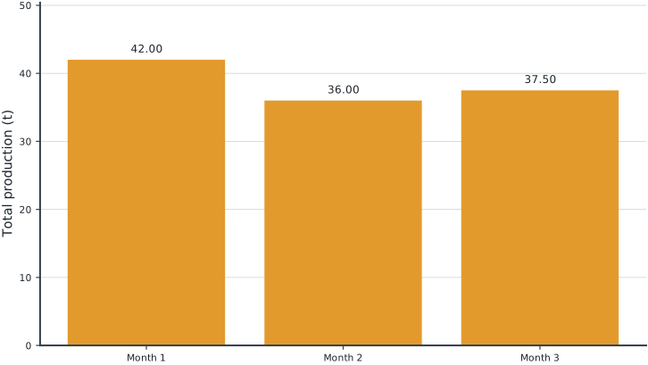
Tables round numerical values for reading; feasibility checks use the original solver values. Multiple optimal decisions may exist. Machine-readable result records the solver status and package versions. Figure-generation code is in figures/workbook.py.
3.5 Brief Discussion
The plan produces 115.50 t and sells 100.50 t; the remaining 15 t satisfy the three terminal stocks.
A capacity reduction can make earlier production and temporary storage worthwhile even though storage has a positive cost. Sales caps are upper bounds, not demand equalities. Experiment: increase month 2 reactor availability by 10 h and calculate the extra contribution; compare it with the cost of overtime.