9 Industrial Capacity Expansion with Intersector Flows
Based on Economic planning, Section 12.9 of Williams (2013). New three-sector industrial-park instance with same-year intermediate inputs and one-year capacity commissioning, explicitly different from the source lags. The results below solve the stated instance and are not presented as the numerical answer to an unmodified textbook problem.
9.1 Problem Statement
An industrial park contains chemicals, utilities, and logistics sectors. Production and capacity are in normalized output units/year. Initial capacities are (100,90,80). The input-output matrix A (row = supplying sector, column = producing sector) is [[0.1,0.2,0.1],[0.3,0.1,0.2],[0.1,0.1,0.1]]. For example, one chemical output unit consumes 0.3 utility units in the same year. Fixed external deliveries are (40,30,20) units each year. One unit of new capacity for a sector requires 0.5 units of that same sector’s output, paid in the construction year; it becomes usable next year. Construction is at most 20 capacity units per sector-year and total labor is at most 110 units/year; production labor coefficients are (0.5,0.4,0.3) and construction requires one labor unit per capacity unit. No output is stored. Over three operating years, maximize capacity available at the end of year 3, including capacity built in year 3 for year 4. Surplus output may be disposed of without credit.
9.1.1 Input coefficients
| Supplying sector | Chemicals output | Utilities output | Logistics output |
|---|---|---|---|
| Chemicals | 0.1 | 0.2 | 0.1 |
| Utilities | 0.3 | 0.1 | 0.2 |
| Logistics | 0.1 | 0.1 | 0.1 |
9.1.2 Sector data
| Sector | Initial capacity | External deliveries | Labor per output unit |
|---|---|---|---|
| Chemicals | 100 | 40 | 0.5 |
| Utilities | 90 | 30 | 0.4 |
| Logistics | 80 | 20 | 0.3 |
9.2 Model Formulation
Production \(x_{it}\ge0\) and additions \(e_{it}\in[0,20]\) are decisions. Available capacity at year \(t\) is \(C_i^0+\sum_{\tau<t}e_{i\tau}\).
\[x_{it}\le C_i^0+\sum_{\tau<t}e_{i\tau},\qquad x_{it}\ge\sum_j A_{ij}x_{jt}+d_i+0.5e_{it}.\] \[\sum_i(l_i x_{it}+e_{it})\le110,\qquad\max\sum_i\left(C_i^0+\sum_t e_{it}\right).\]
Rows of \(A\) describe material availability; columns describe the inputs to one sector’s output. The inequality permits disposal. This LP values all capacity units equally by assumption, so the objective is not monetary welfare.
All decision variables and units refer to the problem statement above. Continuous variables are nonnegative unless explicitly stated otherwise; binary and integer domains are specified in the equations and code.
9.3 Pyomo Implementation
The following Python implementation uses Pyomo and HiGHS. Run from the workbook root so that the models package and shared helpers are importable. The shared solver and audit functions check optimal termination before loading values, then verify every active constraint, variable bound, and integer domain. Any imported earlier-chapter model supplies the data and balances already explained there.
The full source is problem09.py. To solve and print this problem independently:
~/.venvs/optim/bin/python -m models.common 9import pyomo.environ as pyo
from models.common import frame
A = [[0.1, 0.2, 0.1], [0.3, 0.1, 0.2], [0.1, 0.1, 0.1]]
C = [100, 90, 80]
D = [40, 30, 20]
LABOR = [0.5, 0.4, 0.3]
def build():
m = pyo.ConcreteModel()
m.I = pyo.RangeSet(0, 2)
m.T = pyo.RangeSet(0, 2)
m.x = pyo.Var(m.I, m.T, domain=pyo.NonNegativeReals)
m.e = pyo.Var(m.I, m.T, bounds=(0, 20))
m.capacity = pyo.Constraint(
m.I,
m.T,
rule=lambda m, i, t: m.x[i, t] <= C[i] + sum(m.e[i, s] for s in range(t)),
)
m.balance = pyo.Constraint(
m.I,
m.T,
rule=lambda m, i, t: (
m.x[i, t] >= sum(A[i][j] * m.x[j, t] for j in m.I) + D[i] + 0.5 * m.e[i, t]
),
)
m.labor = pyo.Constraint(
m.T, rule=lambda m, t: sum(LABOR[i] * m.x[i, t] + m.e[i, t] for i in m.I) <= 110
)
m.obj = pyo.Objective(
expr=sum(C) + sum(m.e[i, t] for i in m.I for t in m.T), sense=pyo.maximize
)
return m
def check(m):
for t in m.T:
for i in m.I:
net = pyo.value(m.x[i, t]) - sum(
A[i][j] * pyo.value(m.x[j, t]) for j in m.I
)
assert net >= D[i] + 0.5 * pyo.value(m.e[i, t]) - 1e-6
def tables(m):
return {
"plan": frame(
[
[
t + 1,
["Chemicals", "Utilities", "Logistics"][i],
pyo.value(m.x[i, t]),
pyo.value(m.e[i, t]),
C[i] + sum(pyo.value(m.e[i, s]) for s in range(t)),
]
for t in m.T
for i in m.I
],
["Year", "Sector", "Gross output", "Capacity added", "Available capacity"],
)
}
def plot(m):
return (
["Chemicals", "Utilities", "Logistics"],
[C[i] + sum(pyo.value(m.e[i, t]) for t in m.T) for i in m.I],
"Terminal capacity (units/year)",
)
# Solve, audit constraints, and run domain-specific checks.
from models.common import solve, audit
model = solve(build())
audit(model)
check(model)
for name, result_table in tables(model).items():
print(name)
print(result_table.to_string(index=False))9.4 Optimal Solution
The solver reports optimal termination. The objective is 368.67052 capacity units at end of year 3 (maximize). The largest violation across active constraints, variable bounds, and integer domains is 4.44e-15 in the corresponding model units. The problem-specific checks also pass. These checks establish numerical consistency with the stated model, not the validity of its assumptions for a real facility.
9.4.1 Plan
| Year | Sector | Gross output | Capacity added | Available capacity |
|---|---|---|---|---|
| 1 | Chemicals | 66.185 | 0 | 100 |
| 1 | Utilities | 73.4104 | 12.8902 | 90 |
| 1 | Logistics | 48.8439 | 20 | 80 |
| 2 | Chemicals | 66.185 | 0 | 100 |
| 2 | Utilities | 73.4104 | 12.8902 | 102.8902 |
| 2 | Logistics | 48.8439 | 20 | 100 |
| 3 | Chemicals | 66.185 | 0 | 100 |
| 3 | Utilities | 73.4104 | 12.8902 | 115.7803 |
| 3 | Logistics | 48.8439 | 20 | 120 |
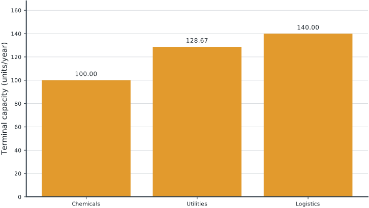
Tables round numerical values for reading; feasibility checks use the original solver values. Multiple optimal decisions may exist. Machine-readable result records the solver status and package versions. Figure-generation code is in figures/workbook.py.
9.5 Brief Discussion
Terminal capacity rises from 270.00 to 368.67 normalized units/year, an addition of 98.67. This objective weights every sector capacity unit equally.
Intersector consumption means gross production exceeds external deliveries. New capacity does not help production in its construction year. Equal weighting of chemically different sectors is a planning convention, not a financial valuation. Experiment: maximize total external sales value instead, specifying a value for each sector and allowing external deliveries to become decisions.