24 Yield Management under Demand Uncertainty
Based on Yield management, Section 12.24 of Williams (2013). New two-stage specialty-chemical campaign sales instance, with a finite price menu and shared first-stage commitments. The results below solve the stated instance and are not presented as the numerical answer to an unmodified textbook problem.
24.1 Problem Statement
A specialty chemical producer may commit to 0, 1, or 2 campaigns, each providing 40 t capacity and costing 70 thousand USD. Before learning later demand, choose an early price of 5 or 4 thousand USD/t; the corresponding early demand limits are 30 and 45 t. Early sales can be rationed. Later demand is low with probability 0.4 or high with probability 0.6. After observing the scenario, choose a later price of 6 or 4 thousand USD/t. Later demand limits at these prices are (20,35) t in the low scenario and (50,70) t in the high scenario. Unsold capacity has no value. Choose first-stage campaigns, early price and early sales, then scenario-specific later prices and sales, to maximize expected revenue minus campaign cost. All production cost is included in the campaign charge.
24.2 Model Formulation
Let integer \(n\in\{0,1,2\}\) be committed campaigns. Early-price binaries \(y_k\) sum to one, and price-indexed early sales \(a_k\) satisfy \(0\le a_k\le D_k y_k\). For each scenario \(s\), later-price binaries \(z_{sk}\) sum to one and sales \(b_{sk}\) satisfy \(0\le b_{sk}\le D_{sk}z_{sk}\).
\[\sum_ka_k+\sum_kb_{sk}\le40n\quad\forall s,\] \[\max\sum_kp_ka_k+\sum_s\pi_s\sum_kP_kb_{sk}-70n.\]
First-stage \(n,y,a\) are shared across scenarios, enforcing nonanticipativity. Later decisions adapt to observed demand. Price-indexed sales avoid multiplying price-choice binaries by a common sales variable.
All decision variables and units refer to the problem statement above. Continuous variables are nonnegative unless explicitly stated otherwise; binary and integer domains are specified in the equations and code.
24.3 Pyomo Implementation
The following Python implementation uses Pyomo and HiGHS. Run from the workbook root so that the models package and shared helpers are importable. The shared solver and audit functions check optimal termination before loading values, then verify every active constraint, variable bound, and integer domain. Any imported earlier-chapter model supplies the data and balances already explained there.
The full source is problem24.py. To solve and print this problem independently:
~/.venvs/optim/bin/python -m models.common 24import pyomo.environ as pyo
from models.common import frame, solve
PROB = [0.4, 0.6]
EARLY = [30, 45]
LATE = [[20, 35], [50, 70]]
EP = [5, 4]
LP = [6, 4]
def build(probabilities=None):
prob = PROB if probabilities is None else probabilities
m = pyo.ConcreteModel()
m.K = pyo.RangeSet(0, 1)
m.S = pyo.RangeSet(0, 1)
m.n = pyo.Var(domain=pyo.Integers, bounds=(0, 2))
m.y = pyo.Var(m.K, domain=pyo.Binary)
m.a = pyo.Var(m.K, domain=pyo.NonNegativeReals)
m.z = pyo.Var(m.S, m.K, domain=pyo.Binary)
m.b = pyo.Var(m.S, m.K, domain=pyo.NonNegativeReals)
m.one = pyo.Constraint(expr=sum(m.y[k] for k in m.K) == 1)
m.later = pyo.Constraint(m.S, rule=lambda m, s: sum(m.z[s, k] for k in m.K) == 1)
m.earlycap = pyo.Constraint(m.K, rule=lambda m, k: m.a[k] <= EARLY[k] * m.y[k])
m.latecap = pyo.Constraint(
m.S, m.K, rule=lambda m, s, k: m.b[s, k] <= LATE[s][k] * m.z[s, k]
)
m.capacity = pyo.Constraint(
m.S, rule=lambda m, s: sum(m.a[k] + m.b[s, k] for k in m.K) <= 40 * m.n
)
m.obj = pyo.Objective(
expr=sum(EP[k] * m.a[k] for k in m.K)
+ sum(prob[s] * LP[k] * m.b[s, k] for s in m.S for k in m.K)
- 70 * m.n,
sense=pyo.maximize,
)
return m
def check(m):
early = sum(pyo.value(m.a[k]) for k in m.K)
assert all(
early + sum(pyo.value(m.b[s, k]) for k in m.K) <= 40 * pyo.value(m.n) + 1e-6
for s in m.S
)
def tables(m):
early = sum(EP[k] * pyo.value(m.a[k]) for k in m.K)
cost = 70 * pyo.value(m.n)
perfect = sum(
PROB[s] * pyo.value(solve(build([1 if j == s else 0 for j in range(2)])).obj)
for s in range(2)
)
return {
"early_commitment": frame(
[
[
pyo.value(m.n),
sum(EP[k] * pyo.value(m.y[k]) for k in m.K),
sum(pyo.value(m.a[k]) for k in m.K),
]
],
["Campaigns", "Early price (thousand USD/t)", "Early sales (t)"],
),
"recourse": frame(
[
[
"Low" if s == 0 else "High",
PROB[s],
sum(LP[k] * pyo.value(m.z[s, k]) for k in m.K),
sum(pyo.value(m.b[s, k]) for k in m.K),
early + sum(LP[k] * pyo.value(m.b[s, k]) for k in m.K) - cost,
]
for s in m.S
],
[
"Scenario",
"Probability",
"Later price (thousand USD/t)",
"Later sales (t)",
"Contribution (thousand USD)",
],
),
"information": frame(
[
["Implementable expected contribution", pyo.value(m.obj)],
["Perfect-information upper bound", perfect],
],
["Measure", "Value (thousand USD)"],
),
}
def plot(m):
t = tables(m)["recourse"]
return (
t["Scenario"].tolist(),
t["Contribution (thousand USD)"].tolist(),
"Scenario contribution (thousand USD)",
)
# Solve, audit constraints, and run domain-specific checks.
from models.common import solve, audit
model = solve(build())
audit(model)
check(model)
for name, result_table in tables(model).items():
print(name)
print(result_table.to_string(index=False))24.4 Optimal Solution
The solver reports optimal termination. The objective is 246 thousand USD expected contribution (maximize). The largest violation across active constraints, variable bounds, and integer domains is 0.00e+00 in the corresponding model units. The problem-specific checks also pass. These checks establish numerical consistency with the stated model, not the validity of its assumptions for a real facility.
24.4.1 Early commitment
| Campaigns | Early price (thousand USD/t) | Early sales (t) |
|---|---|---|
| 2 | 5 | 30 |
24.4.2 Recourse
| Scenario | Probability | Later price (thousand USD/t) | Later sales (t) | Contribution (thousand USD) |
|---|---|---|---|---|
| Low | 0.4 | 4 | 35 | 150 |
| High | 0.6 | 6 | 50 | 310 |
24.4.3 Information
| Measure | Value (thousand USD) |
|---|---|
| Implementable expected contribution | 246 |
| Perfect-information upper bound | 258 |
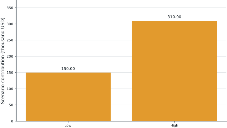
Tables round numerical values for reading; feasibility checks use the original solver values. Multiple optimal decisions may exist. Machine-readable result records the solver status and package versions. Figure-generation code is in figures/workbook.py.
24.5 Brief Discussion
Expected contribution is 246.00 thousand USD. Perfect advance knowledge of demand would raise it to 258.00, so the expected value of perfect information is 12.00 thousand USD.
Expected-value optimization does not mean every scenario earns the expected profit. A first-stage commitment is made before demand is known and must remain feasible in both scenarios. The perfect-information upper bound optimizes first-stage decisions separately for each scenario; it is not an implementable policy. Experiment: change the high-demand probability and identify when the campaign count changes.