7 Mine Operation and Irreversible Closure
Based on Mining, Section 12.7 of Williams (2013). New three-mine, three-year instance, with an explicit minimum blend-quality requirement and irreversible closure. The results below solve the stated instance and are not presented as the numerical answer to an unmodified textbook problem.
7.1 Problem Statement
A mineral processor has three mines A, B, C with annual extraction limits 1.0, 1.2, 0.8 million t; quality indices 1.3, 0.7, 1.1; variable costs 4, 2, 3 million USD per million t; and annual open-mine royalties 1.0, 0.6, 0.8 million USD. At most two mines may operate in a year. Mines are initially open. A mine may remain open while idle, but once closed it cannot reopen. Revenue is 10 million USD per million t sold. Annual sales caps are 1.5, 1.8, 1.2 million t, and minimum blend qualities are 1.0, 1.1, 0.9. Material is blended and sold in the extraction year. Royalty is charged whenever a mine is open. Maximize net present value with all annual cash flows discounted at 10% from each year-end; closure at the start of year 1 is allowed.
7.1.1 Mine data
| Mine | Limit (million t/year) | Quality | Cost (USD/t) | Royalty (million USD/year) |
|---|---|---|---|---|
| A | 1 | 1.3 | 4 | 1 |
| B | 1.2 | 0.7 | 2 | 0.6 |
| C | 0.8 | 1.1 | 3 | 0.8 |
7.1.2 Market data
| Year | Sales cap (million t) | Minimum quality |
|---|---|---|
| 1 | 1.5 | 1 |
| 2 | 1.8 | 1.1 |
| 3 | 1.2 | 0.9 |
7.2 Model Formulation
Use extraction \(x_{it}\ge0\) (million t), operating binary \(a_{it}\), and open binary \(o_{it}\). Let \(U_i,h_i,c_i,R_i,D_t,H_t\) denote capacity, quality, variable cost, royalty, sales cap, and required quality.
\[x_{it}\le U_i a_{it},\quad a_{it}\le o_{it},\quad \sum_i a_{it}\le2,\quad o_{it}\le o_{i,t-1},\quad o_{i0}=1.\] \[\sum_i x_{it}\le D_t,\qquad \sum_i(h_i-H_t)x_{it}\ge0.\] \[\max\sum_{t=1}^3(1.1)^{-t}\left[\sum_i(10-c_i)x_{it}-R_i o_{it}\right].\]
Open and operating are different states. Omitting the open-state variable would allow a mine to avoid royalty in an idle year and reopen later for free.
All decision variables and units refer to the problem statement above. Continuous variables are nonnegative unless explicitly stated otherwise; binary and integer domains are specified in the equations and code.
7.3 Pyomo Implementation
The following Python implementation uses Pyomo and HiGHS. Run from the workbook root so that the models package and shared helpers are importable. The shared solver and audit functions check optimal termination before loading values, then verify every active constraint, variable bound, and integer domain. Any imported earlier-chapter model supplies the data and balances already explained there.
The full source is problem07.py. To solve and print this problem independently:
~/.venvs/optim/bin/python -m models.common 7import pyomo.environ as pyo
from models.common import frame
CAP = [1, 1.2, 0.8]
QUALITY = [1.3, 0.7, 1.1]
COST = [4, 2, 3]
ROYALTY = [1, 0.6, 0.8]
DEMAND = [1.5, 1.8, 1.2]
TARGET = [1, 1.1, 0.9]
def build():
m = pyo.ConcreteModel()
m.I = pyo.RangeSet(0, 2)
m.T = pyo.RangeSet(0, 2)
m.x = pyo.Var(m.I, m.T, domain=pyo.NonNegativeReals)
m.a = pyo.Var(m.I, m.T, domain=pyo.Binary)
m.o = pyo.Var(m.I, m.T, domain=pyo.Binary)
m.c = pyo.ConstraintList()
for t in m.T:
m.c.add(sum(m.a[i, t] for i in m.I) <= 2)
m.c.add(sum(m.x[i, t] for i in m.I) <= DEMAND[t])
m.c.add(sum((QUALITY[i] - TARGET[t]) * m.x[i, t] for i in m.I) >= 0)
for i in m.I:
m.c.add(m.x[i, t] <= CAP[i] * m.a[i, t])
m.c.add(m.a[i, t] <= m.o[i, t])
if t:
m.c.add(m.o[i, t] <= m.o[i, t - 1])
m.obj = pyo.Objective(
expr=sum(
(1.1) ** (-t - 1)
* sum((10 - COST[i]) * m.x[i, t] - ROYALTY[i] * m.o[i, t] for i in m.I)
for t in m.T
),
sense=pyo.maximize,
)
return m
def check(m):
for t in m.T:
total = sum(pyo.value(m.x[i, t]) for i in m.I)
if total > 1e-6:
assert (
sum(QUALITY[i] * pyo.value(m.x[i, t]) for i in m.I) / total
>= TARGET[t] - 1e-6
)
def tables(m):
return {
"schedule": frame(
[
[
t + 1,
"ABC"[i],
pyo.value(m.o[i, t]),
pyo.value(m.a[i, t]),
pyo.value(m.x[i, t]),
]
for t in m.T
for i in m.I
],
["Year", "Mine", "Open", "Operating", "Extraction (million t)"],
)
}
def plot(m):
return (
["Year 1", "Year 2", "Year 3"],
[sum(pyo.value(m.x[i, t]) for i in m.I) for t in m.T],
"Extraction (million t)",
)
# Solve, audit constraints, and run domain-specific checks.
from models.common import solve, audit
model = solve(build())
audit(model)
check(model)
for name, result_table in tables(model).items():
print(name)
print(result_table.to_string(index=False))7.4 Optimal Solution
The solver reports optimal termination. The objective is 20.676935 million USD, discounted to time zero (maximize). The largest violation across active constraints, variable bounds, and integer domains is 0.00e+00 in the corresponding model units. The problem-specific checks also pass. These checks establish numerical consistency with the stated model, not the validity of its assumptions for a real facility.
7.4.1 Schedule
| Year | Mine | Open | Operating | Extraction (million t) |
|---|---|---|---|---|
| 1 | A | 1 | 1 | 0.75 |
| 1 | B | 1 | 1 | 0.75 |
| 1 | C | 1 | 0 | 0 |
| 2 | A | 1 | 1 | 1 |
| 2 | B | 1 | 0 | 0 |
| 2 | C | 1 | 1 | 0.8 |
| 3 | A | 0 | 0 | 0 |
| 3 | B | 1 | 1 | 0.6 |
| 3 | C | 1 | 1 | 0.6 |
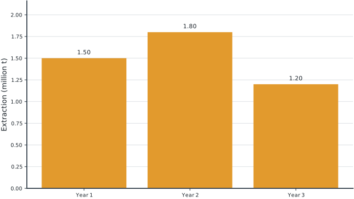
Tables round numerical values for reading; feasibility checks use the original solver values. Multiple optimal decisions may exist. Machine-readable result records the solver status and package versions. Figure-generation code is in figures/workbook.py.
7.5 Brief Discussion
Total extraction is 4.50 million t, with a discounted net value of 20.68 million USD.
Quality makes the high-grade mine valuable even when its extraction cost is larger. An idle-but-open mine pays for future flexibility. The monotone open-state constraint represents permanent closure. Experiment: relax the operation limit from two mines to three and measure the discounted benefit.