11 Robust Calibration by Linear Programming
Based on Curve fitting, Section 12.11 of Williams (2013). New eight-point sensor-calibration dataset; compares straight and quadratic curves under absolute and maximum absolute error. The results below solve the stated instance and are not presented as the numerical answer to an unmodified textbook problem.
11.1 Problem Statement
Calibrate a sensor from input x=[0,1,2,3,4,5,6,7] and response y=[1.0,1.7,2.8,3.1,7.5,4.8,5.5,6.2]. Input and response use normalized laboratory units. Fit (a) a straight line and (b) a quadratic curve, using both minimum total absolute error (L1) and minimum maximum absolute error (L-infinity). No coefficient bounds or monotonicity restrictions are imposed. The unusually large response at x=4 is retained, not silently discarded. The reference objective reported below is the straight-line L1 fit.
11.1.1 Calibration data
| Input | Observed response |
|---|---|
| 0 | 1 |
| 1 | 1.7 |
| 2 | 2.8 |
| 3 | 3.1 |
| 4 | 7.5 |
| 5 | 4.8 |
| 6 | 5.5 |
| 7 | 6.2 |
11.2 Model Formulation
For fixed data \(x_j,y_j\), let \(\hat y_j=a+bx_j+cx_j^2\), setting \(c=0\) for a line. Coefficients are unrestricted real variables. Introduce \(e_j\ge0\) with
\[e_j\ge y_j-\hat y_j,\qquad e_j\ge\hat y_j-y_j.\]
For L1 minimize \(\sum_j e_j\). For L-infinity introduce \(E\ge e_j\) for every observation and minimize \(E\). Both problems are LPs, even for a quadratic curve, because \(x_j^2\) is known data. A curve nonlinear in its input is not necessarily nonlinear in its fitted coefficients.
All decision variables and units refer to the problem statement above. Continuous variables are nonnegative unless explicitly stated otherwise; binary and integer domains are specified in the equations and code.
11.3 Pyomo Implementation
The following Python implementation uses Pyomo and HiGHS. Run from the workbook root so that the models package and shared helpers are importable. The shared solver and audit functions check optimal termination before loading values, then verify every active constraint, variable bound, and integer domain. Any imported earlier-chapter model supplies the data and balances already explained there.
The full source is problem11.py. To solve and print this problem independently:
~/.venvs/optim/bin/python -m models.common 11import pyomo.environ as pyo
from models.common import frame, solve
X = list(range(8))
Y = [1, 1.7, 2.8, 3.1, 7.5, 4.8, 5.5, 6.2]
def build(degree=1, norm="L1"):
m = pyo.ConcreteModel()
m.J = pyo.RangeSet(0, 7)
m.K = pyo.RangeSet(0, degree)
m.beta = pyo.Var(m.K, domain=pyo.Reals)
m.e = pyo.Var(m.J, domain=pyo.NonNegativeReals)
m.E = pyo.Var(domain=pyo.NonNegativeReals)
m.fit = pyo.Expression(
m.J, rule=lambda m, j: sum(m.beta[k] * X[j] ** k for k in m.K)
)
m.pos = pyo.Constraint(m.J, rule=lambda m, j: m.e[j] >= Y[j] - m.fit[j])
m.neg = pyo.Constraint(m.J, rule=lambda m, j: m.e[j] >= m.fit[j] - Y[j])
m.maximum = pyo.Constraint(m.J, rule=lambda m, j: m.E >= m.e[j])
m.obj = pyo.Objective(expr=sum(m.e[j] for j in m.J) if norm == "L1" else m.E)
return m
def check(m):
assert (
abs(sum(abs(Y[j] - pyo.value(m.fit[j])) for j in m.J) - pyo.value(m.obj)) < 1e-6
)
def tables(m):
rows = []
for degree in [1, 2]:
for norm in ["L1", "Linf"]:
a = solve(build(degree, norm))
residual = [abs(Y[j] - pyo.value(a.fit[j])) for j in a.J]
rows.append(
[
degree,
norm,
*[pyo.value(a.beta[k]) if k in a.K else 0 for k in range(3)],
sum(residual),
max(residual),
]
)
return {
"fits": frame(
rows,
["Degree", "Loss", "a", "b", "c", "Total absolute error", "Maximum error"],
),
"observations": frame(
[
[X[j], Y[j], pyo.value(m.fit[j]), Y[j] - pyo.value(m.fit[j])]
for j in m.J
],
["Input", "Observed response", "Reference prediction", "Residual"],
),
}
def plot(m):
return (
[str(x) for x in X],
[Y[j] - pyo.value(m.fit[j]) for j in m.J],
"Reference residual (response units)",
)
# Solve, audit constraints, and run domain-specific checks.
from models.common import solve, audit
model = solve(build())
audit(model)
check(model)
for name, result_table in tables(model).items():
print(name)
print(result_table.to_string(index=False))11.4 Optimal Solution
The solver reports optimal termination. The objective is 4.1 sum of absolute response errors for the reference fit (minimize). The largest violation across active constraints, variable bounds, and integer domains is 6.66e-16 in the corresponding model units. The problem-specific checks also pass. These checks establish numerical consistency with the stated model, not the validity of its assumptions for a real facility.
11.4.1 Fits
| Degree | Loss | a | b | c | Total absolute error | Maximum error |
|---|---|---|---|---|---|---|
| 1 | L1 | 1 | 0.75 | 0 | 4.1 | 3.5 |
| 1 | Linf | 2.5875 | 0.775 | 0 | 13.425 | 1.8125 |
| 2 | L1 | 1 | 0.8029 | -0.0086 | 3.9886 | 3.4257 |
| 2 | Linf | -0.6781 | 2.4 | -0.1937 | 9.1063 | 1.6781 |
11.4.2 Observations
| Input | Observed response | Reference prediction | Residual |
|---|---|---|---|
| 0 | 1 | 1 | 0 |
| 1 | 1.7 | 1.75 | -0.05 |
| 2 | 2.8 | 2.5 | 0.3 |
| 3 | 3.1 | 3.25 | -0.15 |
| 4 | 7.5 | 4 | 3.5 |
| 5 | 4.8 | 4.75 | 0.05 |
| 6 | 5.5 | 5.5 | 0 |
| 7 | 6.2 | 6.25 | -0.05 |
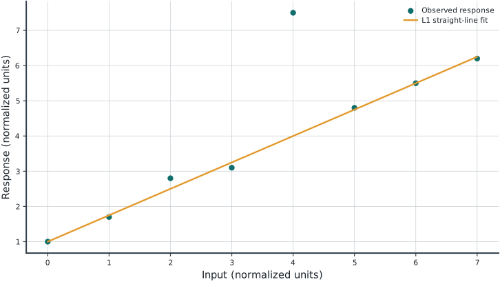
Tables round numerical values for reading; feasibility checks use the original solver values. Multiple optimal decisions may exist. Machine-readable result records the solver status and package versions. Figure-generation code is in figures/workbook.py.
11.5 Brief Discussion
The straight-line L1 fit has total absolute error 4.100 and maximum error 3.500 response units. The table separates these two loss measures.
The L-infinity fit spreads the worst error, while L1 does not square large residuals. Neither method establishes that the high reading is erroneous. The quadratic may improve fit without being a better extrapolation model. Experiment: remove the high observation only as a labeled sensitivity case and compare coefficients.