22 Relative Plant Efficiency by Data Envelopment Analysis
Based on Efficiency analysis, Section 12.22 of Williams (2013). New six-plant dataset with two inputs and one output. Uses input-oriented constant-returns-to-scale DEA. The results below solve the stated instance and are not presented as the numerical answer to an unmodified textbook problem.
22.1 Problem Statement
Compare plants A–F with (energy input, labor input, product output) records A:(100,10,100), B:(120,9,110), C:(110,12,95), D:(140,12,140), E:(100,8,90), F:(150,15,120). Energy is GJ/day, labor is worker-equivalents/day, and output is t/day. Assume comparable products, input quality, operating conditions, and constant returns to scale. Find the maximum proportional input reduction possible for each plant while producing at least its observed output using a nonnegative combination of observed plants. The reported reference objective is the efficiency of Plant C.
22.1.1 Observed plant performance
| Plant | Energy (GJ/day) | Labor (FTE/day) | Output (t/day) |
|---|---|---|---|
| A | 100 | 10 | 100 |
| B | 120 | 9 | 110 |
| C | 110 | 12 | 95 |
| D | 140 | 12 | 140 |
| E | 100 | 8 | 90 |
| F | 150 | 15 | 120 |
22.2 Model Formulation
For target plant \(o\), choose peer weights \(\lambda_j\ge0\) and input-efficiency factor \(\theta\ge0\).
\[\min\theta,\quad\sum_j\lambda_jx_{rj}\le\theta x_{ro}\ (r=\text{energy,labor}),\quad\sum_j\lambda_jy_j\ge y_o.\]
There is no \(\sum_j\lambda_j=1\) constraint under constant returns to scale. The observed plant itself is a feasible comparator, implying \(\theta\le1\) at the optimum. A score of 0.8 means the model finds a comparator producing at least the target output with at most 80% of each target input.
All decision variables and units refer to the problem statement above. Continuous variables are nonnegative unless explicitly stated otherwise; binary and integer domains are specified in the equations and code.
22.3 Pyomo Implementation
The following Python implementation uses Pyomo and HiGHS. Run from the workbook root so that the models package and shared helpers are importable. The shared solver and audit functions check optimal termination before loading values, then verify every active constraint, variable bound, and integer domain. Any imported earlier-chapter model supplies the data and balances already explained there.
The full source is problem22.py. To solve and print this problem independently:
~/.venvs/optim/bin/python -m models.common 22import pyomo.environ as pyo
from models.common import frame, solve
DATA = [
(100, 10, 100),
(120, 9, 110),
(110, 12, 95),
(140, 12, 140),
(100, 8, 90),
(150, 15, 120),
]
def build(target=2):
m = pyo.ConcreteModel()
m.J = pyo.RangeSet(0, 5)
m.lam = pyo.Var(m.J, domain=pyo.NonNegativeReals)
m.theta = pyo.Var(domain=pyo.NonNegativeReals)
m.inputs = pyo.Constraint(
[0, 1],
rule=lambda m, r: (
sum(DATA[j][r] * m.lam[j] for j in m.J) <= m.theta * DATA[target][r]
),
)
m.output = pyo.Constraint(
expr=sum(DATA[j][2] * m.lam[j] for j in m.J) >= DATA[target][2]
)
m.obj = pyo.Objective(expr=m.theta)
return m
def check(m):
assert 0 <= pyo.value(m.theta) <= 1 + 1e-6
assert sum(DATA[j][2] * pyo.value(m.lam[j]) for j in m.J) >= 95 - 1e-6
def tables(m):
rows = []
for o in range(6):
a = solve(build(o))
rows.append(
[
"ABCDEF"[o],
pyo.value(a.theta),
sum(DATA[j][0] * pyo.value(a.lam[j]) for j in a.J),
sum(DATA[j][1] * pyo.value(a.lam[j]) for j in a.J),
]
)
return {
"efficiencies": frame(
rows,
["Plant", "Radial score", "Peer energy (GJ/day)", "Peer labor (FTE/day)"],
),
"reference_peers": frame(
[
["ABCDEF"[j], pyo.value(m.lam[j])]
for j in m.J
if pyo.value(m.lam[j]) > 1e-6
],
["Peer", "Weight for Plant C"],
),
}
def plot(m):
return (
list("ABCDEF"),
[pyo.value(solve(build(o)).theta) for o in range(6)],
"Radial input efficiency",
)
# Solve, audit constraints, and run domain-specific checks.
from models.common import solve, audit
model = solve(build())
audit(model)
check(model)
for name, result_table in tables(model).items():
print(name)
print(result_table.to_string(index=False))22.4 Optimal Solution
The solver reports optimal termination. The objective is 0.863636 input efficiency of Plant C (fraction) (minimize). The largest violation across active constraints, variable bounds, and integer domains is 2.13e-13 in the corresponding model units. The problem-specific checks also pass. These checks establish numerical consistency with the stated model, not the validity of its assumptions for a real facility.
22.4.1 Efficiencies
| Plant | Radial score | Peer energy (GJ/day) | Peer labor (FTE/day) |
|---|---|---|---|
| A | 1 | 100 | 8.5714 |
| B | 1 | 120 | 9 |
| C | 0.8636 | 95 | 8.1429 |
| D | 1 | 140 | 12 |
| E | 0.9419 | 94.186 | 7.5349 |
| F | 0.8 | 120 | 10.2857 |
22.4.2 Reference peers
| Peer | Weight for Plant C |
|---|---|
| D | 0.6786 |
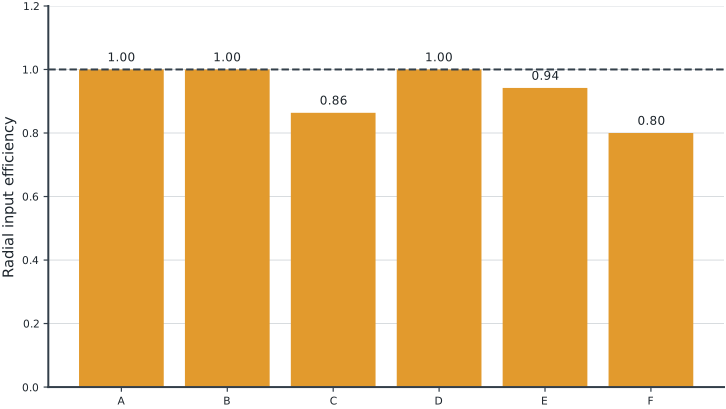
Tables round numerical values for reading; feasibility checks use the original solver values. Multiple optimal decisions may exist. Machine-readable result records the solver status and package versions. Figure-generation code is in figures/workbook.py.
22.5 Brief Discussion
Plant C has radial input efficiency 0.8636, corresponding to a 13.64% proportional input reduction under the constant-returns comparator model.
DEA measures performance relative to this dataset and these assumptions, not thermodynamic efficiency. A radial score of one may still have input or output slack, so it does not alone establish strong efficiency. Experiment: add the convexity constraint on peer weights to obtain variable-returns-to-scale scores and compare them.