21 Dairy Product Pricing with Resource Limits
Based on Agricultural pricing, Section 12.21 of Williams (2013). New four-product instance with finite price menus. This is an exact menu-selection MILP, not a solution of the source continuous-price nonlinear model. The results below solve the stated instance and are not presented as the numerical answer to an unmodified textbook problem.
21.1 Problem Statement
Price milk, butter, cheese A, and cheese B. Baseline prices are (1,4,5,4) thousand USD/t and baseline demands are (100,10,15,10) t/day. Each price must be 0.8, 1.0, or 1.2 times its baseline. Own-price elasticities are (0.4,1.5,1.1,0.4). Demand for product i is its baseline times [1−elasticity_i×(relative price_i−1)]. Each cheese also gains 0.1 times its baseline demand times the other cheese’s relative price increase. Fat fractions are (0.04,0.80,0.35,0.25), and dry-matter fractions are (0.09,0.02,0.30,0.40). Daily available fat and dry matter are 22 and 22 t. All induced demand must be supplied. The price index cannot exceed the baseline: the cost of the baseline basket at new prices must not increase. Maximize daily revenue. Production cost and water availability are outside this exercise.
21.1.1 Product data
| Product | Baseline price (1000 USD/t) | Baseline demand (t/day) | Own elasticity | Fat fraction | Dry fraction |
|---|---|---|---|---|---|
| Milk | 1 | 100 | 0.4 | 0.04 | 0.09 |
| Butter | 4 | 10 | 1.5 | 0.8 | 0.02 |
| Cheese A | 5 | 15 | 1.1 | 0.35 | 0.3 |
| Cheese B | 4 | 10 | 0.4 | 0.25 | 0.4 |
21.2 Model Formulation
Enumerate the 81 price combinations \(k\). For each, calculate prices \(p_{ik}\), induced demands \(d_{ik}\), revenue \(R_k=\sum_i p_{ik}d_{ik}\), fat \(F_k\), dry matter \(M_k\), and baseline-basket expense \(B_k\). Binary \(y_k\) selects exactly one combination:
\[\sum_ky_k=1,\quad\sum_kF_ky_k\le22,\quad\sum_kM_ky_k\le22,\quad\sum_kB_ky_k\le B_0,\] \[\max\sum_kR_ky_k.\]
All menu-dependent quantities are constants, so no product of decision variables remains. This formulation is exact for the stated finite menu only. Increasing menu resolution does not by itself prove global optimality for a continuous pricing model.
All decision variables and units refer to the problem statement above. Continuous variables are nonnegative unless explicitly stated otherwise; binary and integer domains are specified in the equations and code.
21.3 Pyomo Implementation
The following Python implementation uses Pyomo and HiGHS. Run from the workbook root so that the models package and shared helpers are importable. The shared solver and audit functions check optimal termination before loading values, then verify every active constraint, variable bound, and integer domain. Any imported earlier-chapter model supplies the data and balances already explained there.
The full source is problem21.py. To solve and print this problem independently:
~/.venvs/optim/bin/python -m models.common 21import itertools
import pyomo.environ as pyo
from models.common import frame
P = [1, 4, 5, 4]
Q = [100, 10, 15, 10]
E = [0.4, 1.5, 1.1, 0.4]
FAT = [0.04, 0.8, 0.35, 0.25]
DRY = [0.09, 0.02, 0.3, 0.4]
MENUS = list(itertools.product([0.8, 1, 1.2], repeat=4))
def metrics(k):
relative = MENUS[k]
price = [P[i] * relative[i] for i in range(4)]
demand = [
Q[i]
* (
1
- E[i] * (relative[i] - 1)
+ (0.1 * (relative[5 - i] - 1) if i in [2, 3] else 0)
)
for i in range(4)
]
return (
price,
demand,
sum(price[i] * demand[i] for i in range(4)),
sum(FAT[i] * demand[i] for i in range(4)),
sum(DRY[i] * demand[i] for i in range(4)),
sum(price[i] * Q[i] for i in range(4)),
)
def build():
m = pyo.ConcreteModel()
m.y = pyo.Var(range(81), domain=pyo.Binary)
m.one = pyo.Constraint(expr=sum(m.y[k] for k in range(81)) == 1)
m.c = pyo.ConstraintList()
for field, limit in [(3, 22), (4, 22), (5, sum(P[i] * Q[i] for i in range(4)))]:
m.c.add(sum(metrics(k)[field] * m.y[k] for k in range(81)) <= limit)
m.obj = pyo.Objective(
expr=sum(metrics(k)[2] * m.y[k] for k in range(81)), sense=pyo.maximize
)
return m
def check(m):
possible = [
metrics(k)[2]
for k in range(81)
if metrics(k)[3] <= 22 + 1e-9
and metrics(k)[4] <= 22 + 1e-9
and metrics(k)[5] <= 255 + 1e-9
]
assert abs(max(possible) - pyo.value(m.obj)) < 1e-6
def tables(m):
k = next(k for k in range(81) if pyo.value(m.y[k]) > 0.5)
p, d, r, f, s, b = metrics(k)
return {
"pricing": frame(
[
[name, p[i], d[i], p[i] * d[i]]
for i, name in enumerate(["Milk", "Butter", "Cheese A", "Cheese B"])
],
[
"Product",
"Price (thousand USD/t)",
"Demand (t/day)",
"Revenue (thousand USD/day)",
],
),
"resources": frame(
[
["Fat (t/day)", f, 22],
["Dry matter (t/day)", s, 22],
["Basket cost (thousand USD)", b, 255],
],
["Measure", "Use", "Limit"],
),
}
def plot(m):
k = next(k for k in range(81) if pyo.value(m.y[k]) > 0.5)
return ["Milk", "Butter", "Cheese A", "Cheese B"], metrics(k)[1], "Demand (t/day)"
# Solve, audit constraints, and run domain-specific checks.
from models.common import solve, audit
model = solve(build())
audit(model)
check(model)
for name, result_table in tables(model).items():
print(name)
print(result_table.to_string(index=False))21.4 Optimal Solution
The solver reports optimal termination. The objective is 257.6 thousand USD/day (maximize). The largest violation across active constraints, variable bounds, and integer domains is 0.00e+00 in the corresponding model units. The problem-specific checks also pass. These checks establish numerical consistency with the stated model, not the validity of its assumptions for a real facility.
21.4.1 Pricing
| Product | Price (thousand USD/t) | Demand (t/day) | Revenue (thousand USD/day) |
|---|---|---|---|
| Milk | 1 | 100 | 100 |
| Butter | 4 | 10 | 40 |
| Cheese A | 4 | 18.6 | 74.4 |
| Cheese B | 4.8 | 9 | 43.2 |
21.4.2 Resources
| Measure | Use | Limit |
|---|---|---|
| Fat (t/day) | 20.76 | 22 |
| Dry matter (t/day) | 18.38 | 22 |
| Basket cost (thousand USD) | 248 | 255 |
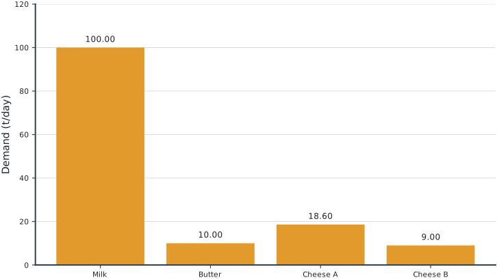
Tables round numerical values for reading; feasibility checks use the original solver values. Multiple optimal decisions may exist. Machine-readable result records the solver status and package versions. Figure-generation code is in figures/workbook.py.
21.5 Brief Discussion
The chosen menu earns 2.60 thousand USD/day more revenue than the baseline price-and-demand combination, subject to the unchanged baseline-basket price-index limit.
Cross-price effects couple the cheese products, while the price index uses baseline quantities rather than the new demand quantities. Revenue is not profit. Experiment: remove the price-index limit and compare both revenue and resource use; then refine the price menu and assess how sensitive the result is to discretization.