23 Two-Day Milk Collection Routing
Based on Milk collection, Section 12.23 of Williams (2013). New six-farm, two-day Euclidean routing instance; retains daily versus alternate-day service and tanker capacity. The results below solve the stated instance and are not presented as the numerical answer to an unmodified textbook problem.
23.1 Problem Statement
A tanker starts and ends at a depot (0,0) on each of two days. Farms 1–6 have coordinates (2,1), (1,4), (4,3), (6,1), (5,5), (2,6) km and collection quantities (3,4,5,4,3,5) thousand L per visit. Farms 1 and 2 are visited every day; farms 3–6 are visited on exactly one of the two days. Quantities for alternate-day farms already represent their per-visit accumulation. Tank capacity is 16 thousand L; there is exactly one tour per day and no intermediate unloading. Travel distance is straight-line Euclidean distance. Minimize two-day distance.
23.1.1 Farm data
| Farm | East (km) | North (km) | Collection (1000 L) | Service |
|---|---|---|---|---|
| 1 | 2 | 1 | 3 | Daily |
| 2 | 1 | 4 | 4 | Daily |
| 3 | 4 | 3 | 5 | Once in two days |
| 4 | 6 | 1 | 4 | Once in two days |
| 5 | 5 | 5 | 3 | Once in two days |
| 6 | 2 | 6 | 5 | Once in two days |
23.2 Model Formulation
Use arc binaries \(x_{ijt}\) for \(i\ne j\), visit binaries \(y_{it}\), and order variables \(u_{it}\) for farms. Depot in-degree and out-degree equal one each day; farm in-degree and out-degree equal \(y_{it}\). Daily farms have \(y_{it}=1\); alternate-day farms have \(\sum_ty_{it}=1\).
\[\sum_iq_i y_{it}\le16,\quad y_{it}\le u_{it}\le6y_{it},\] \[u_{it}-u_{jt}+7x_{ijt}\le6\quad(i,j\ne0,i\ne j).\]
Minimize \(\sum_{ijt}d_{ij}x_{ijt}\). Order constraints eliminate disconnected subtours. They apply only between farms, allowing the tour to return to the depot.
All decision variables and units refer to the problem statement above. Continuous variables are nonnegative unless explicitly stated otherwise; binary and integer domains are specified in the equations and code.
23.3 Pyomo Implementation
The following Python implementation uses Pyomo and HiGHS. Run from the workbook root so that the models package and shared helpers are importable. The shared solver and audit functions check optimal termination before loading values, then verify every active constraint, variable bound, and integer domain. Any imported earlier-chapter model supplies the data and balances already explained there.
The full source is problem23.py. To solve and print this problem independently:
~/.venvs/optim/bin/python -m models.common 23import math
import itertools
import pyomo.environ as pyo
from models.common import frame
COORD = [(0, 0), (2, 1), (1, 4), (4, 3), (6, 1), (5, 5), (2, 6)]
Q = {1: 3, 2: 4, 3: 5, 4: 4, 5: 3, 6: 5}
DIST = {
(i, j): math.dist(COORD[i], COORD[j]) for i in range(7) for j in range(7) if i != j
}
def build():
m = pyo.ConcreteModel()
m.T = pyo.RangeSet(0, 1)
m.I = pyo.RangeSet(1, 6)
m.x = pyo.Var([(i, j, t) for i, j in DIST for t in m.T], domain=pyo.Binary)
m.y = pyo.Var(m.I, m.T, domain=pyo.Binary)
m.u = pyo.Var(m.I, m.T, bounds=(0, 6))
m.c = pyo.ConstraintList()
for t in m.T:
m.c.add(sum(m.x[0, j, t] for j in m.I) == 1)
m.c.add(sum(m.x[j, 0, t] for j in m.I) == 1)
for i in m.I:
m.c.add(sum(m.x[i, j, t] for j in range(7) if j != i) == m.y[i, t])
m.c.add(sum(m.x[j, i, t] for j in range(7) if j != i) == m.y[i, t])
m.c.add(m.u[i, t] >= m.y[i, t])
m.c.add(m.u[i, t] <= 6 * m.y[i, t])
for j in m.I:
if i != j:
m.c.add(m.u[i, t] - m.u[j, t] + 7 * m.x[i, j, t] <= 6)
m.c.add(sum(Q[i] * m.y[i, t] for i in m.I) <= 16)
for i in m.I:
if i <= 2:
for t in m.T:
m.y[i, t].fix(1)
else:
m.c.add(sum(m.y[i, t] for t in m.T) == 1)
m.obj = pyo.Objective(
expr=sum(DIST[i, j] * m.x[i, j, t] for i, j in DIST for t in m.T)
)
return m
def route(m, t):
path = [0]
for _ in range(8):
j = next(
j
for j in range(7)
if j != path[-1] and pyo.value(m.x[path[-1], j, t]) > 0.5
)
path.append(j)
if j == 0:
return path
raise AssertionError("Route did not close")
def check(m):
best = math.inf
def shortest(nodes):
return min(
sum(DIST[a, b] for a, b in zip((0,) + p, p + (0,)))
for p in itertools.permutations(nodes)
)
for mask in itertools.product([0, 1], repeat=4):
groups = [
[1, 2] + [i for i, z in zip(range(3, 7), mask) if z == t] for t in [0, 1]
]
if all(sum(Q[i] for i in group) <= 16 for group in groups):
best = min(best, sum(shortest(group) for group in groups))
assert abs(best - pyo.value(m.obj)) < 1e-6
for t in m.T:
assert len(route(m, t)) == round(sum(pyo.value(m.y[i, t]) for i in m.I)) + 2
def tables(m):
return {
"routes": frame(
[
[
t + 1,
" → ".join(map(str, route(m, t))),
sum(Q[i] * pyo.value(m.y[i, t]) for i in m.I),
sum(DIST[a, b] for a, b in zip(route(m, t), route(m, t)[1:])),
]
for t in m.T
],
["Day", "Tour (0 = depot)", "Collected (1000 L)", "Distance (km)"],
)
}
def plot(m):
return (
["Day 1", "Day 2"],
[sum(DIST[a, b] for a, b in zip(route(m, t), route(m, t)[1:])) for t in m.T],
"Tour distance (km)",
)
# Solve, audit constraints, and run domain-specific checks.
from models.common import solve, audit
model = solve(build())
audit(model)
check(model)
for name, result_table in tables(model).items():
print(name)
print(result_table.to_string(index=False))23.4 Optimal Solution
The solver reports optimal termination. The objective is 33.107398 km over two days (minimize). The largest violation across active constraints, variable bounds, and integer domains is 8.88e-16 in the corresponding model units. The problem-specific checks also pass. These checks establish numerical consistency with the stated model, not the validity of its assumptions for a real facility.
23.4.1 Routes
| Day | Tour (0 = depot) | Collected (1000 L) | Distance (km) |
|---|---|---|---|
| 1 | 0 → 2 → 6 → 5 → 1 → 0 | 15 | 16.7575 |
| 2 | 0 → 1 → 4 → 3 → 2 → 0 | 16 | 16.3499 |
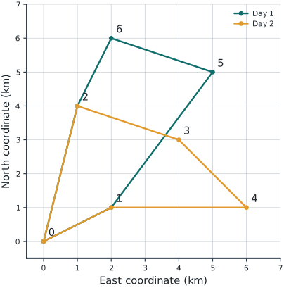
Tables round numerical values for reading; feasibility checks use the original solver values. Multiple optimal decisions may exist. Machine-readable result records the solver status and package versions. Figure-generation code is in figures/workbook.py.
23.5 Brief Discussion
The two tours cover 33.107 km in total. Their collection volumes are 15, 16 thousand L, each within the 16-thousand-L tank limit.
Assigning farms to days and sequencing each tour are coupled by both distance and capacity. Degree constraints alone permit disconnected cycles. Experiment: reduce tank capacity to 15 and determine whether the two-day service pattern remains feasible before interpreting any route.