8 Dairy Farm and Feed Planning

Source and adaptation

Based on Farm planning, Section 12.8 of Williams (2013). New three-year dairy/bioprocess feedstock planning instance. A one-year replacement lag replaces detailed age cohorts. The results below solve the stated instance and are not presented as the numerical answer to an unmodified textbook problem.

8.1 Problem Statement

A dairy feedstock supplier starts with 40 productive cows. Each year 10% leave the herd. The farm may rear 0–8 replacement heifers in years 1 and 2; each joins the productive herd the following year. Herd size during year 1 is fixed at 40. Each productive cow earns net milk contribution of 3 thousand USD/year before feed costs; each heifer reared costs 1.2 thousand USD. Grazing uses 0.5 ha per productive cow and 0.25 ha per heifer. The farm has 40 ha, and remaining land can grow feed at 4 t/ha with growing cost 0.1 thousand USD/ha. Feed demand is 3 t per productive cow and 1 t per heifer; supplemental feed costs 0.2 thousand USD/t. No feed is stored or sold. The year-3 productive herd must be at least 40. Maximize total three-year contribution. Animals are continuous herd-equivalents for strategic planning.

8.2 Model Formulation

Let \(c_t\) be productive herd, \(h_t\) replacements reared, \(a_t\) feed area (ha), and \(f_t\) purchased feed (t).

\[c_1=40,\quad c_{t+1}=0.9c_t+h_t,\quad 0\le h_1,h_2\le8,\quad h_3=0,\quad c_3\ge40.\] \[0.5c_t+0.25h_t+a_t\le40,\quad4a_t+f_t=3c_t+h_t.\] \[\max\sum_t(3c_t-1.2h_t-0.1a_t-0.2f_t).\]

Milk contribution uses the current productive herd, while replacements affect the next year. The terminal herd restriction limits end-of-horizon depletion. The formulation is an LP in expected herd-equivalents.

All decision variables and units refer to the problem statement above. Continuous variables are nonnegative unless explicitly stated otherwise; binary and integer domains are specified in the equations and code.

8.3 Pyomo Implementation

The following Python implementation uses Pyomo and HiGHS. Run from the workbook root so that the models package and shared helpers are importable. The shared solver and audit functions check optimal termination before loading values, then verify every active constraint, variable bound, and integer domain. Any imported earlier-chapter model supplies the data and balances already explained there.

The full source is problem08.py. To solve and print this problem independently:

~/.venvs/optim/bin/python -m models.common 8

import pyomo.environ as pyo
from models.common import frame


def build():
    m = pyo.ConcreteModel()
    m.T = pyo.RangeSet(0, 2)
    m.cows = pyo.Var(m.T, domain=pyo.NonNegativeReals)
    m.heifers = pyo.Var(m.T, bounds=(0, 8))
    m.area = pyo.Var(m.T, domain=pyo.NonNegativeReals)
    m.feed = pyo.Var(m.T, domain=pyo.NonNegativeReals)
    m.cows[0].fix(40)
    m.heifers[2].fix(0)
    m.cows[2].setlb(40)
    m.herd = pyo.Constraint(
        [1, 2], rule=lambda m, t: m.cows[t] == 0.9 * m.cows[t - 1] + m.heifers[t - 1]
    )
    m.land = pyo.Constraint(
        m.T, rule=lambda m, t: 0.5 * m.cows[t] + 0.25 * m.heifers[t] + m.area[t] <= 40
    )
    m.balance = pyo.Constraint(
        m.T, rule=lambda m, t: 4 * m.area[t] + m.feed[t] == 3 * m.cows[t] + m.heifers[t]
    )
    m.obj = pyo.Objective(
        expr=sum(
            3 * m.cows[t] - 1.2 * m.heifers[t] - 0.1 * m.area[t] - 0.2 * m.feed[t]
            for t in m.T
        ),
        sense=pyo.maximize,
    )
    return m


def check(m):
    assert (
        abs(
            pyo.value(m.cows[2])
            - (0.9**2 * 40 + 0.9 * pyo.value(m.heifers[0]) + pyo.value(m.heifers[1]))
        )
        < 1e-6
    )


def tables(m):
    return {
        "plan": frame(
            [
                [
                    t + 1,
                    *[
                        pyo.value(getattr(m, k)[t])
                        for k in ["cows", "heifers", "area", "feed"]
                    ],
                ]
                for t in m.T
            ],
            [
                "Year",
                "Productive herd",
                "Heifers reared",
                "Feed area (ha)",
                "Purchased feed (t)",
            ],
        )
    }


def plot(m):
    return (
        ["Year 1", "Year 2", "Year 3"],
        [pyo.value(m.feed[t]) for t in m.T],
        "Purchased feed (t)",
    )

# Solve, audit constraints, and run domain-specific checks.
from models.common import solve, audit
model = solve(build())
audit(model)
check(model)
for name, result_table in tables(model).items():
    print(name)
    print(result_table.to_string(index=False))

8.4 Optimal Solution

The solver reports optimal termination. The objective is 328.58 thousand USD (maximize). The largest violation across active constraints, variable bounds, and integer domains is 0.00e+00 in the corresponding model units. The problem-specific checks also pass. These checks establish numerical consistency with the stated model, not the validity of its assumptions for a real facility.

8.4.1 Plan

Year	Productive herd	Heifers reared	Feed area (ha)	Purchased feed (t)
1	40	8	18	56
2	44	8	16	76
3	47.6	0	16.2	78

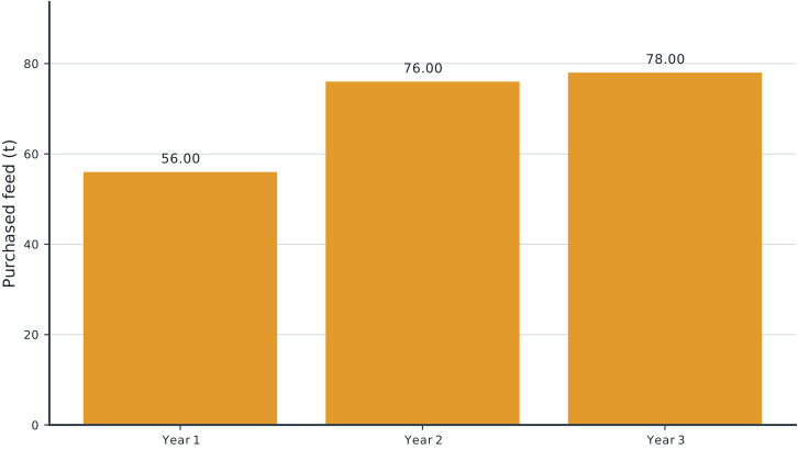
Figure 8.1: Selected quantities from the verified optimal solution. Units are stated on the axis.

Tables round numerical values for reading; feasibility checks use the original solver values. Multiple optimal decisions may exist. Machine-readable result records the solver status and package versions. Figure-generation code is in figures/workbook.py.

8.5 Brief Discussion

The productive herd ends year 3 at 47.60 cow-equivalents. Total supplemental feed purchases are 210.00 t across the three years.

Land links herd growth to purchased-feed expenditure. The replacement lag prevents the model from buying an immediate increase in productive herd through the rearing variable. This simplified model omits age-specific survival and financing. Experiment: remove the terminal herd requirement and quantify the apparent gain from end-of-horizon depletion.