16 Hydro Storage and Thermal Dispatch
Based on Hydro power, Section 12.16 of Williams (2013). Extends the adapted thermal system in Chapter 15 with an energy-equivalent reservoir, pumping losses, and a defined reserve duration. The results below solve the stated instance and are not presented as the numerical answer to an unmodified textbook problem.
16.1 Problem Statement
Add a pumped-hydro unit to Chapter 15. It generates 0–20 MW or pumps at 0–30 MW, but cannot do both in one period. Generation costs 0.1 USD/MWh. Reservoir energy capacity is 240 MWh, with 120 MWh initially and finally. Pumping stores 0.9 MWh per MWh consumed; generating one MWh removes one MWh of stored energy. Reservoir energy at every period-end must be at least 5 MWh so that 20 MW of hydro capability can be available for a 15-minute contingency. Thermal and hydro capability together must cover a 15% demand increase; pumping may be interrupted and hydro can start immediately. No additional hydro startup charge is applied. Minimize total cost, including the thermal costs from Chapter 15. The reserve calculation uses period-end reservoir levels conservatively.
16.2 Model Formulation
Retain thermal power, online states, startups, and their constraints except the original demand and reserve equations. Add hydro generation \(h_t\), pumping \(v_t\), stored energy \(e_t\), and generation-mode binary \(z_t\).
\[\sum_gp_{gt}+h_t=D_t+v_t,\quad 0\le h_t\le20z_t,\quad0\le v_t\le30(1-z_t),\] \[e_t=e_{t-1}+8(0.9v_t-h_t),\quad5\le e_t\le240,\quad e_0=e_3=120.\]
Reserve headroom is \(\sum_g(P_g^{\max}y_{gt}-p_{gt})+(20-h_t)+v_t\). Using the energy balance, requiring it to exceed \(0.15D_t\) is equivalent to \(\sum_gP_g^{\max}y_{gt}+20\ge1.15D_t\). Add \(0.8\sum_t h_t\) to thermal cost. This representation assumes instantaneous pump interruption and hydro availability, supported by the reservoir minimum.
All decision variables and units refer to the problem statement above. Continuous variables are nonnegative unless explicitly stated otherwise; binary and integer domains are specified in the equations and code.
16.3 Pyomo Implementation
The following Python implementation uses Pyomo and HiGHS. Run from the workbook root so that the models package and shared helpers are importable. The shared solver and audit functions check optimal termination before loading values, then verify every active constraint, variable bound, and integer domain. Any imported earlier-chapter model supplies the data and balances already explained there.
The full source is problem16.py. To solve and print this problem independently:
~/.venvs/optim/bin/python -m models.common 16import pyomo.environ as pyo
from models import problem15 as base
from models.common import frame, solve
def build():
m = base.build()
m.balance.deactivate()
m.reserve.deactivate()
m.obj.deactivate()
m.h = pyo.Var(m.T, domain=pyo.NonNegativeReals)
m.pump = pyo.Var(m.T, domain=pyo.NonNegativeReals)
m.e = pyo.Var(m.T, bounds=(5, 240))
m.mode = pyo.Var(m.T, domain=pyo.Binary)
m.hydro = pyo.Constraint(m.T, rule=lambda m, t: m.h[t] <= 20 * m.mode[t])
m.pumping = pyo.Constraint(m.T, rule=lambda m, t: m.pump[t] <= 30 * (1 - m.mode[t]))
m.energy = pyo.Constraint(
m.T,
rule=lambda m, t: (
m.e[t] == (m.e[t - 1] if t else 120) + 8 * (0.9 * m.pump[t] - m.h[t])
),
)
m.e[2].fix(120)
m.new_balance = pyo.Constraint(
m.T,
rule=lambda m, t: (
sum(m.p[g, t] for g in m.G) + m.h[t] == base.DEMAND[t] + m.pump[t]
),
)
m.new_reserve = pyo.Constraint(
m.T,
rule=lambda m, t: (
sum(base.MAX[g] * m.y[g, t] for g in m.G) + 20 >= 1.15 * base.DEMAND[t]
),
)
m.cost = pyo.Objective(expr=m.obj.expr + 0.8 * sum(m.h[t] for t in m.T))
return m
def check(m):
assert (
abs(
sum(pyo.value(m.h[t]) for t in m.T)
- 0.9 * sum(pyo.value(m.pump[t]) for t in m.T)
)
< 1e-6
)
def tables(m):
thermal = solve(base.build())
return {
"storage": frame(
[
[
t + 1,
sum(pyo.value(m.p[g, t]) for g in m.G),
pyo.value(m.h[t]),
pyo.value(m.pump[t]),
pyo.value(m.e[t]),
]
for t in m.T
],
[
"Period",
"Thermal (MW)",
"Hydro (MW)",
"Pumping (MW)",
"Closing energy (MWh)",
],
),
"comparison": frame(
[
["Thermal only", pyo.value(thermal.obj)],
["Thermal and hydro", pyo.value(m.cost)],
],
["System", "Cost (USD/day)"],
),
}
def plot(m):
return (
["Initial", "Period 1", "Period 2", "Period 3"],
[120, *[pyo.value(m.e[t]) for t in m.T]],
"Stored energy (MWh)",
)
# Solve, audit constraints, and run domain-specific checks.
from models.common import solve, audit
model = solve(build())
audit(model)
check(model)
for name, result_table in tables(model).items():
print(name)
print(result_table.to_string(index=False))16.4 Optimal Solution
The solver reports optimal termination. The objective is 7,370.444444 USD/day (minimize). The largest violation across active constraints, variable bounds, and integer domains is 0.00e+00 in the corresponding model units. The problem-specific checks also pass. These checks establish numerical consistency with the stated model, not the validity of its assumptions for a real facility.
16.4.1 Storage
| Period | Thermal (MW) | Hydro (MW) | Pumping (MW) | Closing energy (MWh) |
|---|---|---|---|---|
| 1 | 60 | 0 | 10 | 192 |
| 2 | 120 | 20 | 0 | 32 |
| 3 | 112.2222 | 0 | 12.2222 | 120 |
16.4.2 Comparison
| System | Cost (USD/day) |
|---|---|
| Thermal only | 7,470 |
| Thermal and hydro | 7,370.4444 |
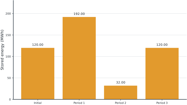
Tables round numerical values for reading; feasibility checks use the original solver values. Multiple optimal decisions may exist. Machine-readable result records the solver status and package versions. Figure-generation code is in figures/workbook.py.
16.5 Brief Discussion
Hydro storage reduces daily operating cost by 99.56 USD. It generates 160.00 MWh and consumes 177.78 MWh for pumping, while restoring the initial stored energy.
Equal initial and final stored energy prevents the optimization from treating the reservoir as free fuel. Pumping loses energy but can shift generation away from costly periods or commitment patterns. Reserve capability and net energy supply are different services. Experiment: set pumping efficiency to one and quantify the value of the avoided loss.