20 Depot Location and Capacity Expansion
Based on Depot location (distribution 2), Section 12.20 of Williams (2013). Extends Chapter 19 with facility fixed costs, an optional D2 expansion, and a two-depot limit. The results below solve the stated instance and are not presented as the numerical answer to an unmodified textbook problem.
20.1 Problem Statement
Use the complete shipping data from Chapter 19. Choose which depots to operate, paying daily fixed costs D1=100, D2=80, D3=60 USD. At most two depots may operate. D2 can be expanded by 20 t/day at an additional 30 USD/day, only if it is open. Other capacities are unchanged. Minimize fixed, expansion, and shipping costs while meeting all customer demands. Fixed costs are daily equivalents of capital and operating commitments; no separate investment horizon is modeled.
20.2 Model Formulation
Add opening binaries \(y_d\) and expansion binary \(e\). Replace depot capacities by
\[\sum_cg_{dc}\le V_d y_d+20e\,\mathbf1_{d=2},\quad e\le y_2,\quad\sum_dy_d\le2.\]
Minimize the transportation objective from Chapter 19 plus \(100y_1+80y_2+60y_3+30e\). A closed depot has zero flow. The expansion term is added capacity, not a multiplication of decision variables, so the formulation remains linear.
All decision variables and units refer to the problem statement above. Continuous variables are nonnegative unless explicitly stated otherwise; binary and integer domains are specified in the equations and code.
20.3 Pyomo Implementation
The following Python implementation uses Pyomo and HiGHS. Run from the workbook root so that the models package and shared helpers are importable. The shared solver and audit functions check optimal termination before loading values, then verify every active constraint, variable bound, and integer domain. Any imported earlier-chapter model supplies the data and balances already explained there.
The full source is problem20.py. To solve and print this problem independently:
~/.venvs/optim/bin/python -m models.common 20import pyomo.environ as pyo
from models import problem19 as base
from models.common import frame
def build():
m = base.build()
m.cap.deactivate()
m.obj.deactivate()
m.y = pyo.Var(m.D, domain=pyo.Binary)
m.e = pyo.Var(domain=pyo.Binary)
m.newcap = pyo.Constraint(
m.D,
rule=lambda m, d: (
sum(m.g[d, c] for c in m.C)
<= base.VD[d] * m.y[d] + (20 * m.e if d == 1 else 0)
),
)
m.requires = pyo.Constraint(expr=m.e <= m.y[1])
m.count = pyo.Constraint(expr=sum(m.y[d] for d in m.D) <= 2)
m.cost = pyo.Objective(
expr=m.obj.expr + sum([100, 80, 60][d] * m.y[d] for d in m.D) + 30 * m.e
)
return m
def check(m):
base.check(m)
for d in m.D:
if pyo.value(m.y[d]) < 0.5:
assert sum(pyo.value(m.g[d, c]) for c in m.C) < 1e-6
def tables(m):
answer = base.tables(m)
answer["facilities"] = frame(
[
[
f"D{d + 1}",
pyo.value(m.y[d]),
pyo.value(m.e) if d == 1 else 0,
sum(pyo.value(m.g[d, c]) for c in m.C),
]
for d in m.D
],
["Depot", "Open", "Expanded", "Throughput (t/day)"],
)
return answer
def plot(m):
return base.plot(m)
# Solve, audit constraints, and run domain-specific checks.
from models.common import solve, audit
model = solve(build())
audit(model)
check(model)
for name, result_table in tables(model).items():
print(name)
print(result_table.to_string(index=False))20.4 Optimal Solution
The solver reports optimal termination. The objective is 615 USD/day (minimize). The largest violation across active constraints, variable bounds, and integer domains is 0.00e+00 in the corresponding model units. The problem-specific checks also pass. These checks establish numerical consistency with the stated model, not the validity of its assumptions for a real facility.
20.4.1 Shipments
| From | To | Flow (t/day) |
|---|---|---|
| P1 | D1 | 45 |
| P2 | D3 | 50 |
| D1 | C1 | 20 |
| D1 | C2 | 25 |
| D3 | C3 | 30 |
| D3 | C4 | 20 |
20.4.2 Facilities
| Depot | Open | Expanded | Throughput (t/day) |
|---|---|---|---|
| D1 | 1 | 0 | 45 |
| D2 | 0 | 0 | 0 |
| D3 | 1 | 0 | 50 |
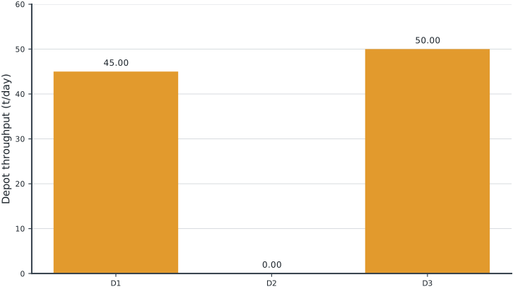
Tables round numerical values for reading; feasibility checks use the original solver values. Multiple optimal decisions may exist. Machine-readable result records the solver status and package versions. Figure-generation code is in figures/workbook.py.
20.5 Brief Discussion
The selected depots are D1, D3. D2 expansion is not selected; total daily cost includes all opening charges.
A fixed charge creates a tradeoff between a more extensive network and cheaper delivery routes. Total capacity alone is necessary but does not explain the best geography. Experiment: remove the two-depot limit and compare the cost-saving value of the third location.