6 Refinery Process and Blend Optimization
Based on Refinery optimisation, Section 12.6 of Williams (2013). New mass-based two-crude teaching instance, with simplified distillation, reforming, cracking, and two final products. The results below solve the stated instance and are not presented as the numerical answer to an unmodified textbook problem.
6.1 Problem Statement
A refinery buys crude A and B at 0.32 and 0.28 thousand USD/t, with daily availability 100 and 80 t. Distillation capacity is 150 t/day. Mass yields (naphtha, gas oil, residue) are (0.5,0.3,0.2) for A and (0.3,0.5,0.2) for B. Naphtha can be blended directly into gasoline with octane index 80 or reformed with mass yield 0.8 to octane-100 reformate. Gas oil can become fuel oil directly or be cracked with yields 0.4 gasoline (octane 95), 0.5 fuel oil, and 0.1 loss. Reforming and cracking feed capacities are 40 and 35 t/day; costs are 0.03 and 0.02 thousand USD/t feed. Residue joins fuel oil. Gasoline must have mass-weighted octane index at least 90. Gasoline and fuel-oil sales limits are 90 and 100 t/day, with prices 0.65 and 0.30 thousand USD/t. All material must be routed or sold; only stated conversion losses leave the system. Maximize daily margin. Linear mass blending of octane is a deliberate teaching approximation.
6.1.1 Crude data
| Crude | Cost (1000 USD/t) | Limit (t/day) | Naphtha yield | Gas-oil yield | Residue yield |
|---|---|---|---|---|---|
| A | 0.32 | 100 | 0.5 | 0.3 | 0.2 |
| B | 0.28 | 80 | 0.3 | 0.5 | 0.2 |
6.2 Model Formulation
Crude feeds \(c_A,c_B\), reformer feed \(r\), cracker feed \(k\), direct naphtha \(n\), and direct gas oil \(d\) are nonnegative t/day. Product sales are \(G,F\).
\[n+r=.5c_A+.3c_B,\quad d+k=.3c_A+.5c_B,\] \[G=n+.8r+.4k,\quad F=d+.5k+.2(c_A+c_B),\] \[80n+100(.8r)+95(.4k)\ge90G.\]
Bound crude feeds by availability, total crude by 150, \(r\le40\), \(k\le35\), \(G\le90\), and \(F\le100\). Maximize \(0.65G+0.30F-0.32c_A-0.28c_B-0.03r-0.02k\). All terms are thousand USD/day. This LP separates unit feed from unit output so conversion losses are not counted twice.
All decision variables and units refer to the problem statement above. Continuous variables are nonnegative unless explicitly stated otherwise; binary and integer domains are specified in the equations and code.
6.3 Pyomo Implementation
The following Python implementation uses Pyomo and HiGHS. Run from the workbook root so that the models package and shared helpers are importable. The shared solver and audit functions check optimal termination before loading values, then verify every active constraint, variable bound, and integer domain. Any imported earlier-chapter model supplies the data and balances already explained there.
The full source is problem06.py. To solve and print this problem independently:
~/.venvs/optim/bin/python -m models.common 6import pyomo.environ as pyo
from models.common import frame
def build():
m = pyo.ConcreteModel()
m.x = pyo.Var(["A", "B", "r", "k", "n", "d", "G", "F"], domain=pyo.NonNegativeReals)
x = m.x
m.c = pyo.ConstraintList()
for key, limit in {"A": 100, "B": 80, "r": 40, "k": 35, "G": 90, "F": 100}.items():
x[key].setub(limit)
m.c.add(x["A"] + x["B"] <= 150)
m.c.add(x["n"] + x["r"] == 0.5 * x["A"] + 0.3 * x["B"])
m.c.add(x["d"] + x["k"] == 0.3 * x["A"] + 0.5 * x["B"])
m.c.add(x["G"] == x["n"] + 0.8 * x["r"] + 0.4 * x["k"])
m.c.add(x["F"] == x["d"] + 0.5 * x["k"] + 0.2 * (x["A"] + x["B"]))
m.c.add(80 * x["n"] + 80 * x["r"] + 38 * x["k"] >= 90 * x["G"])
m.obj = pyo.Objective(
expr=0.65 * x["G"]
+ 0.30 * x["F"]
- 0.32 * x["A"]
- 0.28 * x["B"]
- 0.03 * x["r"]
- 0.02 * x["k"],
sense=pyo.maximize,
)
return m
def check(m):
x = {k: pyo.value(v) for k, v in m.x.items()}
assert abs(x["A"] + x["B"] - x["G"] - x["F"] - 0.2 * x["r"] - 0.1 * x["k"]) < 1e-6
def tables(m):
labels = {
"A": "Crude A",
"B": "Crude B",
"r": "Reformer feed",
"k": "Cracker feed",
"n": "Direct naphtha",
"d": "Direct gas oil",
"G": "Gasoline",
"F": "Fuel oil",
}
return {
"flows": frame(
[[labels[k], pyo.value(v)] for k, v in m.x.items()],
["Stream", "Flow (t/day)"],
)
}
def plot(m):
return (
["Crude A", "Crude B", "Gasoline", "Fuel oil"],
[pyo.value(m.x[k]) for k in ["A", "B", "G", "F"]],
"Flow (t/day)",
)
# Solve, audit constraints, and run domain-specific checks.
from models.common import solve, audit
model = solve(build())
audit(model)
check(model)
for name, result_table in tables(model).items():
print(name)
print(result_table.to_string(index=False))6.4 Optimal Solution
The solver reports optimal termination. The objective is 19.744444 thousand USD/day (maximize). The largest violation across active constraints, variable bounds, and integer domains is 0.00e+00 in the corresponding model units. The problem-specific checks also pass. These checks establish numerical consistency with the stated model, not the validity of its assumptions for a real facility.
6.4.1 Flows
| Stream | Flow (t/day) |
|---|---|
| Crude A | 100 |
| Crude B | 50 |
| Reformer feed | 32.2222 |
| Cracker feed | 35 |
| Direct naphtha | 32.7778 |
| Direct gas oil | 20 |
| Gasoline | 72.5556 |
| Fuel oil | 67.5 |
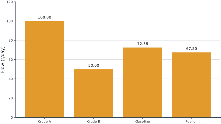
Tables round numerical values for reading; feasibility checks use the original solver values. Multiple optimal decisions may exist. Machine-readable result records the solver status and package versions. Figure-generation code is in figures/workbook.py.
6.5 Brief Discussion
The refinery processes 150.00 t/day and sells 140.06 t/day of products. The 9.94 t/day difference is exactly the modeled conversion loss.
The reformer improves quality but loses mass and incurs cost. More gasoline is therefore not automatically more profitable. The total crude input must equal product sales plus reforming and cracking losses. Experiment: increase gasoline octane to 92 and compare feed selection and conversion intensity.