5 Workforce Planning and Retraining

Source and adaptation

Based on Manpower planning, Section 12.5 of Williams (2013). New two-skill, three-year plant workforce instance; deterministic attrition and continuous full-time equivalents replace the larger source workforce. The results below solve the stated instance and are not presented as the numerical answer to an unmodified textbook problem.

5.1 Problem Statement

A plant initially employs 40 general and 20 skilled full-time equivalents (FTE). At the start of each year 10% of each skill group leaves through natural attrition. After this, the plant may hire, lay off, or train general staff into skilled staff. Training is completed before that year’s operations. Required (general,skilled) FTE in years 1–3 are (30,25), (25,30), (20,35). Annual hiring limits are 8 general and 5 skilled FTE, with costs 3 and 8 thousand USD/FTE. Training costs 4 per FTE, is limited to 6 FTE/year, and can use only surviving general staff, not new hires. Layoffs cost 5 per FTE. Surplus operating staff cost 2 per FTE-year. Ordinary wages are excluded. Minimize total adjustment and surplus cost. FTE are continuous planning averages; no integer headcount interpretation is intended.

5.1.1 Required workforce

Year	General (FTE)	Skilled (FTE)
1	30	25
2	25	30
3	20	35

5.2 Model Formulation

For skill \(g\) and year \(t\), use closing workforce \(w_{gt}\), hires \(h_{gt}\), layoffs \(l_{gt}\), and general-to-skilled training \(v_t\), all nonnegative FTE. With retention \(\rho=0.9\),

\[w_{Gt}=\rho w_{G,t-1}+h_{Gt}-l_{Gt}-v_t,\quad w_{St}=\rho w_{S,t-1}+h_{St}-l_{St}+v_t.\]

Require \(w_{gt}\ge D_{gt}\), hiring limits, \(v_t\le6\), and \(v_t+l_{Gt}\le\rho w_{G,t-1}\). Also \(l_{St}\le\rho w_{S,t-1}\), so newly hired or trained staff are not immediately laid off.

\[\min\sum_t\left[3h_{Gt}+8h_{St}+5\sum_g l_{gt}+4v_t+2\sum_g(w_{gt}-D_{gt})\right].\]

Demand is a minimum staffing requirement. Explicit event timing makes the attrition and training equations unambiguous.

All decision variables and units refer to the problem statement above. Continuous variables are nonnegative unless explicitly stated otherwise; binary and integer domains are specified in the equations and code.

5.3 Pyomo Implementation

The following Python implementation uses Pyomo and HiGHS. Run from the workbook root so that the models package and shared helpers are importable. The shared solver and audit functions check optimal termination before loading values, then verify every active constraint, variable bound, and integer domain. Any imported earlier-chapter model supplies the data and balances already explained there.

The full source is problem05.py. To solve and print this problem independently:

~/.venvs/optim/bin/python -m models.common 5

import pyomo.environ as pyo
from models.common import frame

D = {"G": [30, 25, 20], "S": [25, 30, 35]}
INITIAL = {"G": 40, "S": 20}


def build():
    m = pyo.ConcreteModel()
    m.T = pyo.RangeSet(0, 2)
    m.G = pyo.Set(initialize=["G", "S"])
    m.w = pyo.Var(m.G, m.T, domain=pyo.NonNegativeReals)
    m.h = pyo.Var(m.G, m.T, domain=pyo.NonNegativeReals)
    m.l = pyo.Var(m.G, m.T, domain=pyo.NonNegativeReals)
    m.v = pyo.Var(m.T, bounds=(0, 6))
    m.c = pyo.ConstraintList()
    for t in m.T:
        old = {g: 0.9 * (m.w[g, t - 1] if t else INITIAL[g]) for g in m.G}
        for g in m.G:
            m.c.add(
                m.w[g, t]
                == old[g] + m.h[g, t] - m.l[g, t] + (1 if g == "S" else -1) * m.v[t]
            )
            m.c.add(m.w[g, t] >= D[g][t])
            m.c.add(m.h[g, t] <= (8 if g == "G" else 5))
        m.c.add(m.v[t] + m.l["G", t] <= old["G"])
        m.c.add(m.l["S", t] <= old["S"])
    m.obj = pyo.Objective(
        expr=sum(
            (3 if g == "G" else 8) * m.h[g, t]
            + 5 * m.l[g, t]
            + 2 * (m.w[g, t] - D[g][t])
            for g in m.G
            for t in m.T
        )
        + 4 * sum(m.v[t] for t in m.T)
    )
    return m


def check(m):
    for t in m.T:
        previous = sum(pyo.value(m.w[g, t - 1]) if t else INITIAL[g] for g in m.G)
        assert (
            abs(
                sum(pyo.value(m.w[g, t] - m.h[g, t] + m.l[g, t]) for g in m.G)
                - 0.9 * previous
            )
            < 1e-6
        )


def tables(m):
    return {
        "workforce": frame(
            [
                [
                    t + 1,
                    g,
                    pyo.value(m.w[g, t]),
                    D[g][t],
                    pyo.value(m.h[g, t]),
                    pyo.value(m.l[g, t]),
                ]
                for t in m.T
                for g in m.G
            ],
            [
                "Year",
                "Skill",
                "Workforce (FTE)",
                "Required (FTE)",
                "Hired (FTE)",
                "Laid off (FTE)",
            ],
        ),
        "training": frame(
            [[t + 1, pyo.value(m.v[t])] for t in m.T], ["Year", "Retrained (FTE)"]
        ),
    }


def plot(m):
    return (
        ["Year 1", "Year 2", "Year 3"],
        [pyo.value(m.v[t]) for t in m.T],
        "Retrained staff (FTE)",
    )

# Solve, audit constraints, and run domain-specific checks.
from models.common import solve, audit
model = solve(build())
audit(model)
check(model)
for name, result_table in tables(model).items():
    print(name)
    print(result_table.to_string(index=False))

5.4 Optimal Solution

The solver reports optimal termination. The objective is 130.5 thousand USD (minimize). The largest violation across active constraints, variable bounds, and integer domains is 0.00e+00 in the corresponding model units. The problem-specific checks also pass. These checks establish numerical consistency with the stated model, not the validity of its assumptions for a real facility.

5.4.1 Workforce

Year	Skill	Workforce (FTE)	Required (FTE)	Hired (FTE)
1	G	30	30	0
1	S	25	25	1
2	G	25	25	4
2	S	30	30	1.5
3	G	20	20	3.5
3	S	35	35	2

5.4.2 Training

Year	Retrained (FTE)
1	6
2	6
3	6

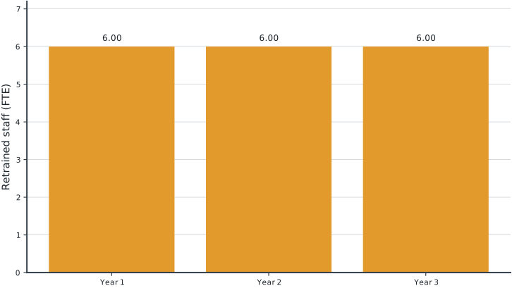
Figure 5.1: Selected quantities from the verified optimal solution. Units are stated on the axis.

Tables round numerical values for reading; feasibility checks use the original solver values. Multiple optimal decisions may exist. Machine-readable result records the solver status and package versions. Figure-generation code is in figures/workbook.py.

5.5 Brief Discussion

The solution retrains 18.00 FTE over three years and lays off 0.00 FTE. Hiring and training jointly cover the changing skill mix.

Retraining preserves workforce while meeting a shift toward skilled operations, but its cost must be compared with hiring, attrition, and temporary surplus. Fractional FTE are acceptable for strategic averages; a detailed roster would need integer people and a different attrition treatment. Experiment: halve training capacity and measure the cost increase.