17 Three-Dimensional Binary Pattern Design
Based on Three-dimensional noughts and crosses, Section 12.17 of Williams (2013). Retains the 3×3×3 grid and the 13/14 split. Interpreted as a combinatorial modeling exercise, not a physical reactor model. The results below solve the stated instance and are not presented as the numerical answer to an unmodified textbook problem.
17.1 Problem Statement
Place 13 white and 14 dark markers in a 3×3×3 grid, one per cell. A line consists of three equally spaced cells on a straight grid direction: axes, face diagonals, or body diagonals. There are 49 such lines. Minimize the number of lines whose three markers have the same color. This exercise teaches counting violations of a discrete pattern, which can also appear in equipment assignment or experimental layout.
17.2 Model Formulation
Binary \(x_i=1\) denotes a white marker. For each line \(\ell\), introduce \(z_\ell\in[0,1]\) and write
\[\sum_i x_i=13,\quad z_\ell\ge\sum_{i\in\ell}x_i-2,\quad z_\ell\ge1-\sum_{i\in\ell}x_i.\]
Minimize \(\sum_\ell z_\ell\). When a line contains zero or three white markers, the corresponding lower bound forces \(z=1\). Otherwise, minimization sets it to zero. The penalty variables can be continuous even though the cell assignments must be binary.
All decision variables and units refer to the problem statement above. Continuous variables are nonnegative unless explicitly stated otherwise; binary and integer domains are specified in the equations and code.
17.3 Pyomo Implementation
The following Python implementation uses Pyomo and HiGHS. Run from the workbook root so that the models package and shared helpers are importable. The shared solver and audit functions check optimal termination before loading values, then verify every active constraint, variable bound, and integer domain. Any imported earlier-chapter model supplies the data and balances already explained there.
The full source is problem17.py. To solve and print this problem independently:
~/.venvs/optim/bin/python -m models.common 17import itertools
import pyomo.environ as pyo
from models.common import frame
CELLS = list(itertools.product(range(3), repeat=3))
LINES = sorted(
{
tuple(
sorted(
(
p,
tuple(p[k] + d[k] for k in range(3)),
tuple(p[k] + 2 * d[k] for k in range(3)),
)
)
)
for p in CELLS
for d in itertools.product([-1, 0, 1], repeat=3)
if any(d) and all(0 <= p[k] + 2 * d[k] <= 2 for k in range(3))
}
)
def build():
assert len(LINES) == 49
m = pyo.ConcreteModel()
m.x = pyo.Var(CELLS, domain=pyo.Binary)
m.z = pyo.Var(range(len(LINES)), bounds=(0, 1))
m.count = pyo.Constraint(expr=sum(m.x[i] for i in CELLS) == 13)
m.c = pyo.ConstraintList()
for j, line in enumerate(LINES):
total = sum(m.x[i] for i in line)
m.c.add(m.z[j] >= total - 2)
m.c.add(m.z[j] >= 1 - total)
m.obj = pyo.Objective(expr=sum(m.z[j] for j in range(len(LINES))))
return m
def check(m):
white = {i for i in CELLS if pyo.value(m.x[i]) > 0.5}
assert len(white) == 13
mono = sum(len(set(line) & white) in [0, 3] for line in LINES)
assert abs(mono - pyo.value(m.obj)) < 1e-6
def tables(m):
return {
"grid": frame(
[[*i, "White" if pyo.value(m.x[i]) > 0.5 else "Dark"] for i in CELLS],
["x", "y", "z", "Marker"],
)
}
def plot(m):
return (
["Layer 0", "Layer 1", "Layer 2"],
[sum(pyo.value(m.x[i]) for i in CELLS if i[2] == z) for z in range(3)],
"White markers in layer",
)
# Solve, audit constraints, and run domain-specific checks.
from models.common import solve, audit
model = solve(build())
audit(model)
check(model)
for name, result_table in tables(model).items():
print(name)
print(result_table.to_string(index=False))17.4 Optimal Solution
The solver reports optimal termination. The objective is 4 monochromatic straight lines (minimize). The largest violation across active constraints, variable bounds, and integer domains is 8.88e-15 in the corresponding model units. The problem-specific checks also pass. These checks establish numerical consistency with the stated model, not the validity of its assumptions for a real facility.
17.4.1 Grid
| x | y | z | Marker |
|---|---|---|---|
| 0 | 0 | 0 | Dark |
| 0 | 0 | 1 | White |
| 0 | 0 | 2 | Dark |
| 0 | 1 | 0 | White |
| 0 | 1 | 1 | White |
| 0 | 1 | 2 | Dark |
| 0 | 2 | 0 | Dark |
| 0 | 2 | 1 | Dark |
| 0 | 2 | 2 | White |
| 1 | 0 | 0 | White |
| 1 | 0 | 1 | Dark |
| 1 | 0 | 2 | White |
| 1 | 1 | 0 | White |
| 1 | 1 | 1 | White |
| 1 | 1 | 2 | Dark |
| 1 | 2 | 0 | Dark |
| 1 | 2 | 1 | White |
| 1 | 2 | 2 | Dark |
| 2 | 0 | 0 | Dark |
| 2 | 0 | 1 | White |
| 2 | 0 | 2 | White |
| 2 | 1 | 0 | White |
| 2 | 1 | 1 | Dark |
| 2 | 1 | 2 | Dark |
| 2 | 2 | 0 | Dark |
| 2 | 2 | 1 | Dark |
| 2 | 2 | 2 | White |
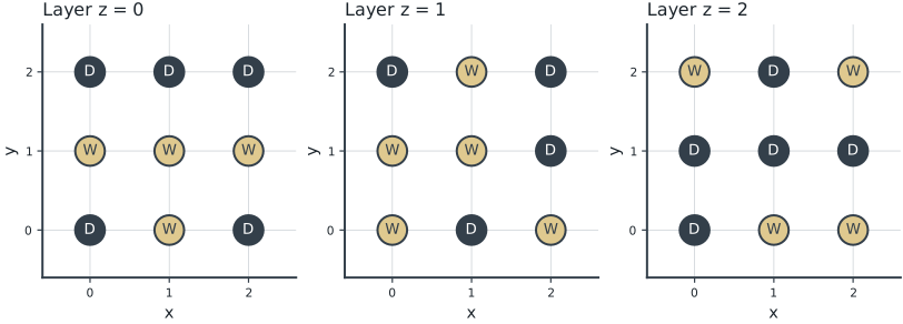
Tables round numerical values for reading; feasibility checks use the original solver values. Multiple optimal decisions may exist. Machine-readable result records the solver status and package versions. Figure-generation code is in figures/workbook.py.
17.5 Brief Discussion
The optimum has 4 monochromatic lines among the 49 possible lines, with exactly 13 white markers.
A local pattern penalty can be linearized without listing every complete grid. The 49-line generation must avoid duplicate directions, or the objective gives some patterns extra weight. Experiment: change the white-marker count and plot the minimum penalty as a function of that count.